Author: IMC

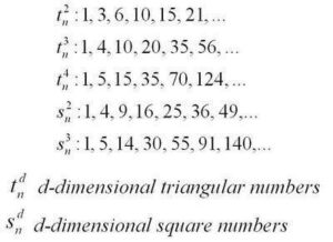
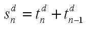
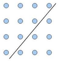
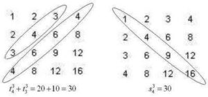
There is a nice identity stating that a square number can be written as the sum of two subsequent triangular numbers.

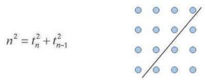
Here we are writing tdn for the nth triangular of dimension d (d=2 are the flat polygonals, d=3 for they pyramidal polygonals, etc.)

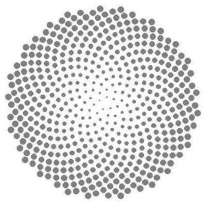
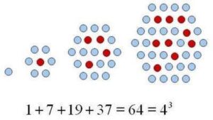
There is also a nice relationship that connects cubes to polygonal numbers. It turns out that a cube of spheres can be unfolded into a packed-hexagonal pyramid. The “packed hexagonals” or “centered hexagonals” are not quite the usual hexagonal numbers – instead these are hexagons of dots with the gaps filled in. The picuture below shows how square numbers fill the gaps of the hexagonals perfectly to form the “packed hexagonals,” and how these in turn can be stacked to form a cube. Here we are using phdn for “packed hexagonals” hdn for hexagonals, sdn for squares, and tdn for triangular numbers.

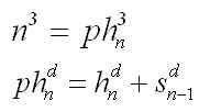
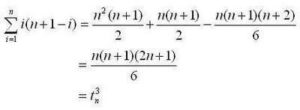
Combining this result with the “triangulation” identities we have:

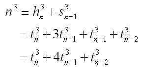
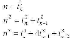
This gives us three nice identities for powers of n:

It turns out that these identities generalize for other positive integer powers of n. Every nd can be written as a sum of tdi where i ranges from n to n+1−d. (for any i less than 1, these terms are zero)

1.Write out the sequence of nd for at least 2d−2 terms. Take the finite difference of this sequence d−2 times (this reduces the sequence down to “2-dimensional” numbers, allowing us to use the 2-dimensional triangular numbers in our calculations).

2.The first term of the new sequence should be 1. Eliminate the first term by subtracting t2n from this sequence. This means that our sum begins with tdn, with a coefficient of 1. Ensure that the t2n values are subtracted from the corresponding terms of the sequence.

3. Now, the sequence has a new first term which is A. Eliminate this term by subtracting A t2n from the sequence. A is the coefficient of tdn−1.

4. Repeat step 3, eliminating the first term of the sequence each time with a multiple of t2n, which provides the coefficient for the next value of tdi.

5.The process ends when all terms in the nd sequence is eliminated, which happens at the dth step.

Carrying out this process for a few more powers of n, we end up with:

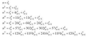
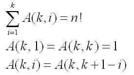
In general, we seem to have:

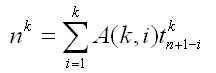
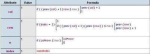
where the coefficients A(i,k) have the nice properties:

The coefficients are naturally analogous to the binomial coefficients, and can be arranged in a triangle like Pascal’s.

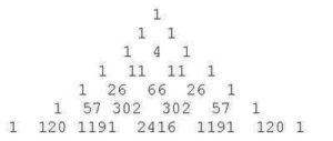
These coefficients are known as Eulerian numbers, and the construction above is known as Euler’s Number Triangle (not to be confused with the geometric construction called the Euler Triangle).

For more such insights, log into www.international-maths-challenge.com.

*Credit for article given to dan.mackinnon*

If mathematics is a game, then playing some game is doing mathematics, and in that case why isn’t dancing mathematics too?

Ludwig Wittgenstein – Remarks on the Foundations of Mathematics

Mathematics is often described metaphorically – the  forms that these metaphors take include the organic, mechanical, classical, and post-modern, among countless others. Within these metaphors, mathematics may be a tool, or set of tools, a tree, part of a tree, a vine, a game, or set of games, and mathematicians in turn may be machines, game-players, artists, inventors, or explorers.

Despite the many metaphors used to describe mathematics, in popular discourse mathematics is often reduced to one of its parts, being metonymically described as merely about numbers, formulas, or some other limited aspect. Metaphor is a more complete substitution of ideas than metonymy – allowing us to link concepts that do not appear to have any direct relationship. Perhaps, metaphoric language that elevates and expands our ideas about mathematics is used by enthusiasts to counter the more limited and diminishing metonymic descriptions that are often encountered.

Attempts to describe and elevate mathematics through metaphor seem to fall short, however. Our usual way of thinking about things is to inquire about their meaning – a meaning that is assumed to lie beneath or beyond mere appearances. Metaphor generally relies on making connections between concepts on this deeper level. The sheer formalism of mathematics frustrates this usual way of thinking, and leaves us grasping for a meaning that is constantly evasive. The sheer number and variety of the  many metaphors for mathematics suggests that no single convincing one has yet been found. It may be that the repeated attempts to find such a unifying metaphor represents an ongoing and forever failing attempt to grapple with the purely formal character of mathematics; and it may be that the formal nature of mathematics will always shake off any metaphor that attempts to tie it down.

For more such insights, log into www.international-maths-challenge.com.

*Credit for article given to dan.mackinnon*

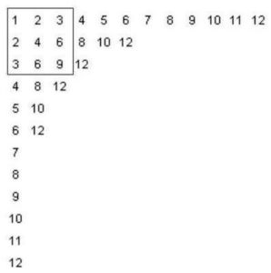
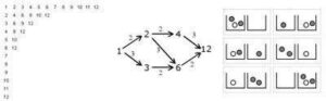
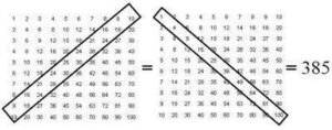A surprising relationship found in the multiplication table is that the sum of the entries in the main upwards diagonal and the diagonal above it is equal to the sum of the entries in the main downwards diagonal. What is also surprising is that this is but one among several observations about the multiplication table that can be expressed in terms of polygonal numbers.

This relationship involves three-dimensional triangular numbers (triangle-based pyramidal numbers, or tetrahedral numbers), and three-dimensional square numbers (square-based pyramidal numbers). Some values for these, and a few other polygonals, are shown below.

To see why this relationship holds, first note that the sum of the entries in the nth upward diagonal in the multiplication table is equal to the nth three-dimensional triangular number.

Second, observe that he entries in the main down diagonal are square numbers (two-dimensional), so the sum of the main down diagonal is the nth three-dimensional square number.

Finally, we use the fact that a square number (of any dimension) can be split into two triangular numbers (of the same dimension), which gives us the surprising result above.

the image below shows the relationship for a 4×4 multiplication table.

For more such insights, log into www.international-maths-challenge.com.

*Credit for article given to dan.mackinnon*

The names of the trigonometric ratios tangent and secant are derived from the Latin “to touch” and “to cut” – the tangent to a figure is a line that touches it in one place, where a secant cuts through it in two or more. But how are these geometric terms related to the ratios that bear their names? The answer can be shown using the diagram at the top of the post – a diagram that used to be a standard one in high school trig text books.

Consider the acute angle BAC. Allow |AC| = 1, and construct a unit circle about A that goes through C. Construct a tangent to this circle at C, and extend the segment AB so that it meets this tangent at E. So, the segment CE lies on the tangent while the segment AE lies on the secant of the unit circle formed around BAC. ACE is a new right triangle that contains the original BAC.

The tangent of BAC is BC/AB (opposite/adjacent), but if we now look at the second triangle ACE, we see tht it is also given by (CE/AC)=(CE/1)=CE – the tangent is measured by the segment of the tangent, CE. Similarly, the secant of BAC is given by AC/AB (hypoteneuse/adjacent), but again turning to the second triangle ACE, we see that this is (AC/AB)=(AE/AC)=(AE/1)=AE – and the secant is provided by the length of the secant, AE.

This treatment was taken from the book “Plane Trigonometry and Tables” by G. Wentworth, published in 1903. In some of the texts of this era, the “primary” trigonometric ratios were sin, sec, and tan (rather than sin, cos, and tan), perhaps owing their primacy to constructions like the one described above.

The cosine was considered a secondary trigonometric ratio – its name coming from the phrase “complement’s sine.” Along with the usual ratios, texts often presented several convienience ratios that are now antiquated, such as the versedsine vrsin(x) = 1-cos(x) and the half-versed sine or haversine hvrsn(x)= (1/2)vrsin(x).

The most fundamental trigonometric ratio has the most obscure name. It is generally claimed that the word “sine” comes from Latin word for “bend,” but some have suggested that the word is ultimately derived from the name of the curve formed by the gathering of a toga, or from the Latin word for “bowstring.” In Arithmetic, Algebra, Analysis, Felix Klein states that “sine” represents a Latin mis-translation of an Arabic word, but does not go on to explain its origins any further.

For more such insights, log into www.international-maths-challenge.com.

*Credit for article given to dan.mackinnon*

In many traditions, Biedermann’s Dictionary of Symbols tells us, “the tree was widely seen as the axis mundi around which the cosmos is organized” and, as mentioned in a previous post, has been widely used to describe the relationship between mathematics and other sciences. Mathematics itself, like many subjects, is often portrayed as a tree whose sub-topics make up branches that continue to grow and bifurcate.

Some recent articles have take a more postmodern perspective on using the tree metaphor to describe mathematics.

Dan Kennedy ‘s “Climbing around on the Tree of Mathematics,” (full text here) and Greg McColm’s “A Metaphor for Mathematics Education” are two recent articles that make arguments by analogy about what mathematics is and how it should be taught. In Kennedy’s argument, mathematics is a tree, while in McColm’s it is a vine – both are organic, growing, and branching. What distinguishes these two uses of metaphor from traditional tree analogies is that both authors are not at all suggesting that we can stand back and survey the structure as a whole and understand how all its parts are related. The ability to provide a comprehensive view of the subject, to make it surveyable, was the raison-d’être of metaphors like the “Tree of Science.” Instead of using the metaphor this way, both authors suggest that we think of ourselves as part of the growing structure – as climbers and gardeners who cannot see the complex organic whole, but who can explore and tend to our small part of it. In these descriptions, natural forms like trees and plants, once metaphors for simplicity and comprehensibility, now provide metaphors for complexity.

Up in the Tree of Mathematics, Kennedy suggests that working mathematicians are labouring at extending its outer branches. This is where the view is best, where the fruit is found, and where the beauty of mathematics can be seen most clearly. School Mathematics is part of the trunk, the solid, oldest, stable part of the tree, and math teachers spend their time helping students climb the trunk, hoping that some may one day reach its outer branches. Unfortunately, the difficulty of the trunk prevents most people from ever climbing beyond it. Kennedy suggests that we should be less concerned with the trunk than with the branches, and that technology can provide a ladder to assist the climb.

McColm’s Mathematical Vine is not mathematics itself, but a structure that clings to the underlying reality of mathematical truth. Mathematics, in this analogy, is like a hidden tower, whose shape can only be seen by looking at the vine that has taken shape around it. Like in Kennedy’s analogy, working mathematicians are the caretakers who help the structure grow. For McColm, this analogy emphasizes the importance of mathematics education – a process of strengthening the vine so that it may continue to grow. Perhaps because his audience is primarily post-secondary researchers, he does not advocate finding shortcuts to “higher” views, but rather suggests that education be promoted through “tending to the vine” – clarifying mathematics and strengthening connections between different branches.

Although they suggest more of a structure at play, rather that a stable unified whole, organic metaphors like those used by McColm and Kennedy continue to suggest a natural unity among the various parts of mathematics. In that sense they are still rooted (or centered), and, although they have somewhat destabilized the tree analogy, they haven’t quite deconstructed it. They have not, for example, gone quite as far as Wittgenstein, who seemed to suggest that metaphors that attempt to link the subjects of mathematics in a defining way like this are misguided. In his view, as described by Ackerman (1988, p. 115):

mathematics is an assemblage of language games, having no sharp and uniform external boundary, with potentially confusing and criss-crossing subdisciplines held together by an internal network of analogous proof techniques.

It is easy to appreciate how some climbers in Kennedy’s trees and McColm’s vines end up like the protagonist in Roz Chast’s cartoon “Falling off the Math Cliff”, where step 1 is “A boy begins his wondrous journey,” and step 8 is “The plummet.”

The images in this post are “Pythagoras Tree” fractals, made using GSP.

For more such insights, log into www.international-maths-challenge.com.

*Credit for article given to dan.mackinnon*

When asked to describe mathematics we often resort to metaphor rather than attempt to provide strict definitions. These pictures from high school math textbooks from the 1930s are an example of this tendancy.

The simple hierarchies of these images resolve the complicated relationship between mathematics and science by appealing to our desire for an organic unity among disciplines, giving mathematics a foundational role within the general concept of science. These images are appealing, but do not stand up to scrutiny.

The simple relationship between mathematics and science becomes complicated when mathematics is described, as it sometimes is, as a science itself. It’s definition as “the science of space and quantity” is further complicated by the caveat that it is an exact deductive science, unlike the usual inductive kind. Following this line of thinking further, mathematics is then described as a kind of meta-science, or a limit point to which science might aspire – science emptied of all of its empirical content, a science of pure thought. While some view mathematics as a foundation for science, others as a supra-science, the emerging field of experimental mathematics brings mathematics back into the empirical fold, reducing it (or elevating it) to a science like any other. So, mathematics can be seen as root, branch, or even the form of the tree itself.

Thinking about these things for even a short while evokes some sympathy with Bertrand Russell’s remark that “mathematics may be defined as the subject in which we never know what we are talking about, nor whether what we are saying is true.”

For more such insights, log into www.international-maths-challenge.com.

*Credit for article given to dan.mackinnon*

Start with a square piece of paper (like a Post it note), fold and unfold it in half along a mid-line or along a diagonal. Take another identical square, and fold and unfold it the same way. Decide on some way to place the second square on the first, so that the second is somewhat rotated. Use only the edges of the square and the creases that you made to determine the placement. Make your placement precise so that your “rule” can be described exactly in terms of the edges and creases. Repeat this process, placing a third square on top of your second square using exactly the same rule. Repeat until your placing of papers leads you back to the first piece.

The resulting construction might look something like the one shown on the left below. If you take your papers, set them in place with some careful light gluing, and place them on a window, the sunlight passing through the overlapping papers creates a stained-glass effect that shows a variety of shapes.

This sort of construction is a simplified version of what William Gibbs describes in his book “Window Patterns.” In Gibbs’ treatment, the pattern is partially planned in advance, and then the dimensions of the rectangular pieces of paper that make up the pattern are determined using a little trigonometry. This process can be simplified by starting with a more limited range of options for paper dimension and placement. It turns out that a surprising number of window patterns can be created by only using squares, their mid-lines, and their diagonals, and that these patterns invariably have “special triangles” and related regular polygons and star-polygons embedded within them.

Here are a two more “placement rules” and the patterns that they give rise to.

The diagrams were created using Geometer’s Sketchpad – if you construct the rule using translations applied to a constructed square, you can use the iteration feature to create the final pattern. GSP provides a good environment for planning out the patterns prior to constructing them with paper, and building the plans in GSP is enjoyable and instructive as well.

For more such insights, log into www.international-maths-challenge.com.

*Credit for article given to dan.mackinnon*

Starting with p (p a positive integer) equally distributed dots (vertices) around a circle. Connecting each dot to the next as you move around the circle will give you a regular p-gon – a p-sided polygon with p vertices. If, however, instead of connecting each dot to the one next to it you skip over a fixed number of dots, then you might end up with a star-like pattern, like the ones shown above. In this process, imagine that you start with a particular vertex and move in a counter-clockwise direction. If there are any dots left-over when you get back to the dot you started from, just throw away the unconnected dots.

The Schläfli notation for polygons is very useful for describing regular connected star polygons, and provides an example of how sometimes calculations with notation match exactly with calculations done with diagrams. In this notation, regular polygons like triangle, square, pentagon, etc. are written as {3}, {4}, and {5} respectively. A regular p-gon is written as {p}. If when drawing your p-gon you connect to the second next vertex instead of the first, then you would write this as {p/2}. If you connect to the q’th next vertex, then you would write this polygon as {p/q}. Note that if you are just connecting to the next vertex to make a regular p-gon, this notation gives you {p/1} = {p}, as you would expect.

If you start playing with this process you will notice that {p/q} gives you the same polygon as {p/(p–q)} (as long as you ignore the orientation of the polygon). You may also notice that if q is larger than p, you end up repeating the same patterns, in particular {p/q} = {p/(q mod p)}. Also you will notice that if p and q have common factors, you end up having skipped vertices. In our process we are throwing these away to ensure that our polygons are connected, but you can extend the process and keep them (see note below).

The process described is straightforward to implement in a program. The images shown here were generated in Tinkerplots. To implement it in Tinkerplots, you need two sliders – p and q, and the following attributes:

n = caseIndex()
theta = 2*n*pi(1-q/p)
x = cos(theta)
y = sin(theta)

If you create a plot with y vertical and x horizontal, choose “show connecting lines” and add a filter n<=p+1, you can add a large number of cases to the collection (~200, say) and be able to slide p and q to create a wide variety of connected star polygons. The only restriction is that p must be less than the number of cases you have created. There is nothing special about using Tinkerplots here – any programming environment with reasonable graphics should do a reasonable job (Logo would be fine. :)).

The polygons below are the regular connected polygons based on 12 vertices. Because 12 is divisible by 2, 3, 4, and 6 we end up with regular polygons triangle {3}, square {4}, hexagon {6} and only one star polygon {12/5}. The “degenerate” polygon {2} is known as a “digon.” Here, drawing the diagram first and then seeing what polygon comes out will give you the same result as dividing p/q first and then drawing the corresponding polygon. In this sense, the notation and diagrams nicely reflect each other.

Contrast this with the family of star polygons that are generated when a prime number of vertices are used. The images below are the family of regular connected polygons generated on 13 vertices.

Note – by throwing away the unconnected dots in our process we are ignoring star polygons that are made of overlapping disjoint star or regular polygons, for example two overlapping triangles that make a star of David. These also work well with the Schläfli notation. To create these overlapping polygons, if you have any skipped vertices, you just begin your process again beginning with one of the vertices you skipped over. In the case of {6/2}, instead of getting one triangle {3} you will get two overlapping triangles, or 2{3}. To write a program that would draw these you would want to use something more sophisticated than Tinkerplots.

For more such insights, log into www.international-maths-challenge.com.

*Credit for article given to dan.mackinnon*

A surprisingly interesting structure is the extended multiplication table, shown above for the numbers seven to ten. The algorithm for drawing these is straight forward – for an n-extended table, start out as if you were writing a “regular” multiplication table, but extend each row so that it gets as close to, without exceeding, n. Another way to think about it is to write out rows of “skip counting up to n” by i for integers i from 1 to n.

This is called an extended multiplication table since it contains a “traditional” multiplication table inside it. The 12-extended table below contains a traditional 3×3 multiplication table.

It turns out that 1 appears in an extended table once, and prime numbers appear exactly twice (once in the first column, and once in the first row). In general, for a natural number n, how many times does n appear in the n-extended table?

Before looking at that question, you might want to think about finding easier ways to draw the tables. Drawing out these tables by hand can be tedious – a simple program or spreadsheet might be easier. You can use Fathom, for example, to create the table data and draw it in the collections display. Create a slider m and the attributes listed in the table below (click on the image to see a larger version).

Modify the collection display attributes to draw the tables in the collection box. By adding lots of cases and using the slider m to filter out the ones you don’t need, you can vary the size of the table easily.

“how many times does n appear in the n-extended table?”

# of occurrances of n in the n-extended table = # of nodes in the factor lattice Fn

You can also recast both of these questions (how many occurances of n in the n-extended table, and how many nodesin the Fn factor lattice) as a combinatorial “balls in urns” problem.

Consider a set of colored balls where there are m different colours, where there are ki balls of color i, where i ranges from 1 to m. This would give a total number of balls equal to k1+k2+…+km. Suppose you were to distribute these balls in two urns. How many different distributions would there be? Using some counting techniques, you will find that the answer is (k1+1)*(k2+1)*…*(km+1).

How is this connected to the other problems? Consider the prime factorization of the number. For each prime, choose a colour, and for each occurance of the prime in the factorization, add a new ball of that color. For example for 12 = 3*3*2, choose two colours – say blue=3 and red=2. Since 3 occurs twice and 2 occurs once, there should be two blue balls and one red ball. Now consider distributing these balls in two urns. It turns out that you get (2+1)*(1+1) = 6 possibilities. This is the same number of times 12 occurs in the 12-extended table, and the same number of nodes in the 12-factor lattice. The image below shows the 12-extended table, the 12-factor lattice, and the “ball and urn problem” for the numer 12.

For a number n with the prime factorization:

The answer to all three questions is given by:

For more such insights, log into www.international-maths-challenge.com.

*Credit for article given to dan.mackinnon*

If you have already created the phyllotaxis data in Fathom, or opened the data created in TinkerPlots in Fathom, you can change the display you get when you drag open a collection box. Under the display tab on the Collection Inspector in Fathom you can set the display properties so that cases no longer show up as uniform gold balls. Setting the display attributes to the values below should give you a growing spiral like the one pictured above.

x = 10x+400
y = 10y+400
image = greyCircleIcon
width = sqrt(r*10)
height = sqrt(r*10)
caption=””

Note that the x and y on the right-hand side of the equations above are the x and y attributes that you defined for the data, and the x and y on the left-hand correspond to the position of the icons. You can experiment with other formulas for width and height—using a slider to provide a variable instead of the number “10” gives more flexibility.

The images below show some of the other spirals you can obtain by varying the angle between the seeds, as mentioned in the previous post.

For more such insights, log into www.international-maths-challenge.com.

*Credit for article given to dan.mackinnon*