Author: IMC

The triangular numbers (and higher triangular numbers) can be generated using this recurrence relationship:

These will form Pascal’s triangle (if we shift the variables n->n+d-1 and d->r, we get the familiar C(n,r) indexing for the Pascal Triangle). The d=2 case gives the usual “flat” 2d triangular numbers, and other d values provide triangular numbers of different dimensions.

 

It turns out that recurrence relation can be generalized to generate a family of sequences and triangles. Consider this more general relation:

Doing some initial exploring reveals four interesting cases:

The triangular numbers 

With all these additional parameters set to 1, we get our original relation, the familiar triangular numbers, and Pascal’s triangle.

The k-polygonal numbers 

If we set the “zero dimension” to k-2, we end up with the k-polygonal numbers. The triangular numbers arise in the special case where k=3. Except in the k=3 case, the triangles that are generated are not symmetrical.

 

Below is the triangle generated by setting k=5.

The symmetrically shifted k-polygonal numbers

As far as I know, there is not a standard name for these.  Each k value will generate a triangle that is symmetrical about its center and whose edge values are equal to k-2. For a given k value, if you enter sequences generated by particular values of d, you’ll find that some are well known. The codes in the diagrams correspond to the sequence ids from the Encyclopedia.

 

Here is the triangle generated by k=4:

And here is the triangle generated for k=5:

The Eulerian numbers (Euler’s number triangle)

This is a particularly nice way to generate the Eulerian numbers, which have a nice connection to the triangular numbers. There is a little inconsistency in the way the Eulerian numbers are indexed, however. For this formula to work, it should be altered slightly so that d>0. The resulting formula looks like this:

And the triangle looks like this:

It is surprising that so many interesting and well known sequences and triangles can be generated from such a simple formula, and that they can be interpreted as being part of a single family.

For more such insights, log into www.international-maths-challenge.com.

*Credit for article given to dan.mackinnon*

There are plenty of probability problems that have counter-intuitive solutions. Problems like these, and how they can undermine common sense, are among the best reasons for looking at probability theory. One set of humbling questions is the family of Monty Hall problems. Another are those related to conditional probability; nice examples of these are problems that involve medical tests that give ‘false positive’ results.

Simulation is a way of exploring these problems that reveals more than mere theoretical probability calculations do. The structure of the simulation can reflect interesting aspects of the structure of the original problem, and the results reveal a variability that is not apparent when you simply calculate the theoretical probabilities on their own.

This post shows an example of a ‘false positive’ probability problem and a Fathom simulation for it. This problem was adapted from one found in the 4th edition of Ross’s A First Course in Probability (p.75):

A laboratory blood test is 95 percent effective in detecting a certain disease when it is, in fact, present. However, the test also yields a “false positive” result for one percent of healthy persons. (That is, if a healthy person is tested, there is a 0.01 probability that they will test positive for the disease, even though they don’t really have it.) If 0.5 percent of the population actually has the disease, what is the probability that a person who has a positive test result actually has the disease?

Here are the attribute definitions that you could use to build a Fathom simulation for this problem:

The attributes are enough to run the simulation, but it is better to also add the following measures:

To run the simulation you can add new cases (try ~500). Using a measures collection, you can re-run this experiment hundreds of times (collecting a 100 measures re-runs the 500 person experiment 100 times).

If you are calculating the theoretical probability by hand, it helps to write down all of the probabilities (fill in the blanks…):

It also helps to visualize the probabilities in a tree diagram:

The outer tips of the tree are filled in using the multiplicative rule for conditional probabilities:

One nice thing about doing this is that you can see how the tree diagram used to calculate the theoretical probabilities is structured in the same way as the “if” statements in the simulation.

For more such insights, log into www.international-maths-challenge.com.

*Credit for article given to dan.mackinnon*

Students generally learn to divide polynomials using  long division or synthetic division. This post is about another method for dividing polynomials,  the “grid” method. Although this method is used at some schools, I have not found it in any textbook (if you know of any, please let me know).

The grid method makes polynomial division a fun calculation – an almost SUDOKU-like process. The recreational challenge here is to master the method, and to convince yourself that it actually works in all cases (which cases does it work well for, and which are more difficult?).

Before tackling polynomial grid division, you need to be familiar with polynomial grid multiplication. It is the symbolic analog to the familiar “algebra tiles” manipulative, so if you have worked with these, it should be reasonably familiar.

Polynomial Grid Multiplication

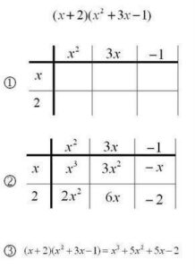
In polynomial grid multiplication, the two factors are arranged on the edges of a grid – the number of terms of the factors determine the number of horizontal and vertical lines that make up the grid.

The overall product is found by filling in the cells of the grid with the product of the terms for the row and column, and then summing up all the contents of the interior of the grid.

What polynomial grid multiplication does for us is provide an explicit way to keep track of the distributive property: each term-by-term product gets its own cell.

In the example below, the two factors are placed along the edges of the grid (1). One factor provides the row headings, the other provides the column headings. Then each cell is filled in with the product of the terms from the row and column (2). Finally, the cells are added together (like terms are combined) to find the final product (3). If the terms of the factors are placed according to the same order (descending powers of x, in our example) and there are no missing terms, then like-terms of the product are found along the diagonals of the grid.

Polynomial Grid Division

Polynomial grid division works the same way as polynomial grid multiplication, but in reverse – we start by knowing one of the factors (placed along the edge of the grid), and by knowing what we want the product to be (without knowing exactly how it is ‘split up’ in the grid). Using this knowledge we work backwards, filling in the grid and the top edge one cell at a time until we are done.

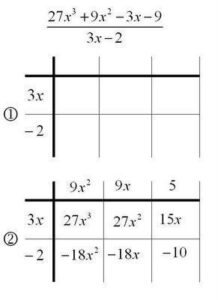
Consider the example below. In (1) we create an empty grid with the denominator (divisor) playing the role of one of the factors. Since this question involves a degree 3 polynomial divided by a degree 1 polynomial, we know that the other factor (the quotient) must be degree 2. This allows us to create a grid with the correct size. In step (2) we use the highest power of the dividend (the numerator) to begin to fill in the grid – we know that 27x^3 must be in the top left. This in turn tells us that the first column entry must be 9x^2 (so that the row and column multiply to 27x^3). In step (3) we use this to fill in all of the first column, multiplying 9x^2 by the terms of the row entries.

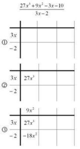
In step (3) we now have a quadratic term -18x^2. But we know from looking at the dividend (numerator) that in the final answer we actually want 9x^2. Consequently, the other entry on the quadratic diagonal must be 27x^2, so that the whole diagonal sums to 9x^2 .  Filling this in for step (4) tells us what all the entries in the second column should be (step 5). Now that we have a linear entry -18x, we know that we need to add in a 15x so that the overall sum gives a -3x (step 6).

Having a 15x tells us that the top entry must be 5 (the product of 5 and 3x gives us 15x). Filling this in in step 7 allows us to complete the table, and we see that our final constant entry is -10, as hoped for. Now that the grid has been filled in and it matches the dividend, we can read the answer off the top – the factor that we have uncovered is the quotient we were hoping to calculate.

This method is actually easier than it seems at first, and when all steps are carried out on the same grid, is quite compact.

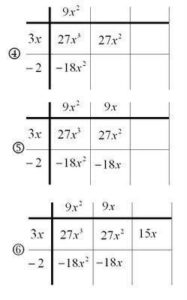
Here is another example for you to try it out on.

In these two examples, the division worked well – there was no remainder. In the case where we are dividing f/g and g is not a factor of f, and the degree of g is less than the degree of f, there is polynomial remainder whose degree is strictly less than that of g. So, for example, when g is a linear function (degree 1), f/g can have a constant remainder (degree 0).

In this case we proceed as above, attempting to fill in the grid with the numerator (dividend). However, if when we are done the grid does not match the numerator, we have a remainder. The remainder is the additional amount that we have to add to the grid in order to arrive at the numerator.

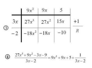
Consider a division question almost identical to the first one that we looked at, except here we change the numerator slightly so that it doesn’t factor well.

Following the same steps as before, we end up with a grid sum that does not match our desired answer: we have -10 instead of -9 for the final constant term. This tells us that we have a remainder of +1, that we choose to write next to the grid. In our final answer, the remainder tells us the “remaining fractional part” that we have to add at the end.

For more such insights, log into www.international-maths-challenge.com.

*Credit for article given to dan.mackinnon*

Here is an outline of how you can go about generating this data. The definition and properties of Farey sequences here are from Hardy & Wright’s An Introduction to the Theory of Numbers (which I am slowly working my way through).
The Farey sequence of order n is the sequence of irreducible fractions between 0 and 1 whose denominator does not exceed n. So, the elements of the sequence are of the form h/k, where h < k < n, and h and k are relatively prime.

The main theorem about Farey numbers provides them with their characteristic property (Theorem 29 in TofN). The characteristic property of Farey sequences is that if h/k, h”/k”, and h’/k’ are successive terms in a Farey sequence, then h”/k” is the mediant of h/k and h’/k’. If h/k and h’/k’ are two reduced fractions, their mediant is given by (h+h’)/(k+k’).

It’s nice when a theorem tells you how to implement an algorithm. This property tells us that Farey sequences can be built iteratively or recursively, beginning with F1={0/1 ,1/1}. The algorithm to do this is a nice one – it’s probably not often used as a textbook exercise in recursion because it helps if you to have some data structure or class to represent the fraction, and a way of telling if integers are relatively prime (you can use the Euclidean algorithm to implement a gcd() function).

Here is an outline of how to calculate the next Farey sequence, given that you have one already.

0) input a Farey sequence oldSequence (initial sequence will be {0/1, 1/1})

1) create a new empty sequence newSequence

2) iterate over oldSequence and find out its level by finding the largest denominator that occurs store this in n

3) set n= n+1

4) iterate over oldSequence, looking at each pair of adjacent elements (left and right)

4.1) add left to newSequence
4.2) if the denominators of left and right sum to n, form their mediant
4.2.1) if the numerator and denominator of the mediant are relatively prime, add mediant to newSequence

5) add the last element of oldSequence to newSequence

Note that you only need to add in new elements where the denominators of existing adjacent elements sum to the n value – when this happens you form the mediant of the two adjacent elements. Furthermore, the mediant is only added if the fraction can’t be reduced.

Below is some Java-ish code corresponding to the above – it assumes that the oldSequence and newSequence are an ArrayList and that you have a class Fraction that has fields num (numerator) and den (denominator).

Here are the first five Farey sequences that you get from the algorithm:

The image at the top of the post was generated by implementing the algorithm in Processing, and using the result to draw the associated Ford circles – you could do something similar in regular Java (or other language). If you draw the Ford Circles associated with the sequence, the circle for a fraction “frac” will be centered at (x,y) and have a radius r where

x = (scale)*frac.num/frac.den

y = r

r = (scale)/(2*(frac.den)^2)

where “scale” is some scaling factor (probably in the 100’s) that increases the size of the image.

Here I decided to draw two copies of each circle, one on top of the other.

 

That it contains only fractions between 0 and 1 and that it contains all reduced fractions for denominators k < n, connects Farey sequences to Euler’s totient function. Euler’s totient function is an arithmetic function that for a given k, counts the integers less than k that are relatively prime to it. This is exactly the number of times that a fraction of the form h/k will appear in the Farey sequence for k>1.

The Farey algorithm, how to draw Ford circles, and the connection to Euler’s totient function are described nicely in J.H. Conway and R.K. Guy’s The Book of Numbers – a great companion to a book like TofN.

 

For more such insights, log into www.international-maths-challenge.com.

*Credit for article given to dan.mackinnon*

 

Chapter 3 of Hardy & Wright’s An Introduction to the Theory of Numbers involves Farey sequences – which, in addition to showing up in serious number theory books, are an interesting, accessible, and popular topic in recreational mathematics.

Since I am a committed constructivist (in at least a few senses of the word) I thought it would be nice to come up with an activity with Farey sequences that could be carried out without too much advance discussion about what they are. What I came up with is a Fathom activity that starts with some simple but odd looking data that allows you to construct some very interesting plots and displays. The idea is that you will get a feel for what a Farey sequence is by using the data to build the sequence and by looking at the results from different perspectives.

Step 1. Import some data

Here is the data to import into Fathom. It should create 33 cases with two attributes n, and d.

n d

0 1

1 10

1 9

1 8

1 7

1 6

1 5

2 9

1 4

2 7

3 10

1 3

3 8

2 5

3 7

4 9

1 2

5 9

4 7

3 5

5 8

2 3

7 10

5 7

3 4

7 9

4 5

5 6

6 7

7 8

8 9

9 10

1 1

 

Step 2. Add some more attributes

After importing this data, you should create the following attributes

i = caseIndex

q = n/d

dist = q – prev(q)

mediant = (n+prev(n))/(d+prev(d))

d_mediant = mediant – prev(mediant)

disp = concat(n,”/”,d)

The meaning of the “mediant” attributes will become clearer after you read about Farey sequences.

 

Step 3. Explore some plots

Plots you could try creating are:

1. A) n on the y axis and d on the x axis.
2. B) dist on y, i on x (a filter of i>1 makes sense here)
3. C) d_mediant on y, i on x (a filter of i>2 makes sense here)
4. D) mediant on y, q on x (adding a function y=x makes sense here)
5. E) d on y, q on x
6. F) dist on y, q on x
7. H) q on x with no other attributes

While creating these plots, you should be thinking about describing the sequence that the cases represent. What kinds of numbers are they, what values do they have (do they lie in a certain interval?), how close are they to one another?

Step 4. Create a nice display

One of the more visually interesting thing you can do with the Farey sequence is to display its associated Ford circles. This can be done by adding two new sliders and by editing the display settings for the collection.

 

Add the sliders “scale” and “shift,” and give them these initial values:

scale = 400

shift = 150

Now on the collection inspector, click on the Display tab, and edit the formulas for these attributes

x= q*scale +shift

y = scale/(2*d^2)

image = blueCircleIcon

width = scale/(d^2)

height = scale/(d^2)

caption = “”

If you pull open the display, you will see the initial iterations of a fractal pattern known as the Ford Circles that are generated by the Farey sequence. Here is what it should look like:

For more such insights, log into www.international-maths-challenge.com.

*Credit for article given to dan.mackinnon*

The double recurrence relation that defines the higher triangular numbers is a simple one – it is no surprise that they turn up so often.

The geometric interpretation is stacking: For a given dimension d, you get the n+1 d-triangular number by stacking the nth d-1 triangular number (the gnomon) onto the nth d-triangular number.  The zero dimensional triangular numbers are just the sequence: 1, 1, 1, 1,…, presumably counting stacks of nothing. The one-dimensional triangular numbers are the naturals: 1, 2, 3, 4, …, made by stacking the ones of the one-dimensional case. The two dimensional triangular numbers stack the naturals: 1, 3, 6, 10, …, the three dimensional triangular numbers make pyramids of the triangulars: 1, 4, 10, 20, ….

If you write out a difference table for the higher triangular numbers, you end up with Pascal’s triangle. This suggests a nice formula for the triangulars in terms of binomial coefficients:

From this, you can obtain another recursive formula that you can use when working with higher triangular numbers (this is the “another” formula for this post):

If you vary the defining recurrence relation so that the initial “zero dimensional” value is a number other than 1, you get the other polygonal numbers (square, pentagonal, hexagonal, square-based pyramidal, etc.). In particular, if you let the zero-dimensional value be k-2, you obtain the k-polygonal numbers (k-2 corresponding to the number of triangles in your k-sided polygon).

It turns out there is a nice formula for these in terms of binomial coefficients as well:

For more such insights, log into www.international-maths-challenge.com.

*Credit for article given to dan.mackinnon*

As I make my way through Hardy & Wright’s An Introduction to the Theory of Numbers,  I am hoping to work it into my recreational math pursuits – coming up with interesting (but not too heavy) activities that correspond roughly to the material in the text.

The first two chapters are on the sequence of primes. Here’s the activity: obtain a list of primes, import them into Fathom, and construct plots that explore pn and pi(n) and other aspects of the sequence that manifest themselves in the first couple of thousand terms.

In my Fathom experiment, I imported the first 2262 prime numbers.

If you import a sequential list of primes into Fathom (under the attribute prime) and add another attribute n=caseindex, you can create two nice plots. Plot A should have prime as the x axis and n  as the y axis. This shows the function pi(n). To this plot you should add the function y = x/ln(x) and visually compare the two curves. Plot B should have the x and y axis reversed. On this graph, plotting the function y = x*ln(x) shows how closely this approximation for pn (the nth prime) comes to the actual values.

 

You can add further attributes to look at the distance between primes dist=prime-prev(prime), and also the frequency of twin primes is_twin = (dist=2)or(next(dist)=2).

You can also add attributes to keep a running count of twin_primes, and to keep a running average of the twin_primes. The plot above shows how the ratio of tiwn primes diminishes as the number of primes increases. The plot at the top of the post suggests the distribution of primes and twin primes (in blue) in the numbers up to the 2262nd prime.

For more such insights, log into www.international-maths-challenge.com.

Credit for article given to dan.mackinnon*

There is a nice identity stating that a square number can be written as the sum of two subsequent triangular numbers.

Here we are writing tdn for the nth triangular of dimension d (d=2 are the flat polygonals, d=3 for they pyramidal polygonals, etc.)

There is also a nice relationship that connects cubes to polygonal numbers. It turns out that a cube of spheres can be unfolded into a packed-hexagonal pyramid. The “packed hexagonals” or “centered hexagonals” are not quite the usual hexagonal numbers – instead these are hexagons of dots with the gaps filled in. The picuture below shows how square numbers fill the gaps of the hexagonals perfectly to form the “packed hexagonals,” and how these in turn can be stacked to form a cube. Here we are using phdn for “packed hexagonals” hdn for hexagonals, sdn for squares, and tdn for triangular numbers.

Combining this result with the “triangulation” identities we have:

This gives us three nice identities for powers of n:

It turns out that these identities generalize for other positive integer powers of n. Every nd can be written as a sum of tdi where i ranges from n to n+1−d. (for any i less than 1, these terms are zero)

1.Write out the sequence of nd for at least 2d−2 terms. Take the finite difference of this sequence d−2 times (this reduces the sequence down to “2-dimensional” numbers, allowing us to use the 2-dimensional triangular numbers in our calculations).

2.The first term of the new sequence should be 1. Eliminate the first term by subtracting t2n from this sequence. This means that our sum begins with tdn, with a coefficient of 1. Ensure that the t2n values are subtracted from the corresponding terms of the sequence.

3. Now, the sequence has a new first term which is A. Eliminate this term by subtracting A t2n from the sequence. A is the coefficient of tdn−1.

4. Repeat step 3, eliminating the first term of the sequence each time with a multiple of t2n, which provides the coefficient for the next value of tdi.

5.The process ends when all terms in the nd sequence is eliminated, which happens at the dth step.

Carrying out this process for a few more powers of n, we end up with:

In general, we seem to have:

where the coefficients A(i,k) have the nice properties:

The coefficients are naturally analogous to the binomial coefficients, and can be arranged in a triangle like Pascal’s.

These coefficients are known as Eulerian numbers, and the construction above is known as Euler’s Number Triangle (not to be confused with the geometric construction called the Euler Triangle).

For more such insights, log into www.international-maths-challenge.com.

*Credit for article given to dan.mackinnon*

 

If mathematics is a game, then playing some game is doing mathematics, and in that case why isn’t dancing mathematics too?

Ludwig Wittgenstein – Remarks on the Foundations of Mathematics

Mathematics is often described metaphorically – the  forms that these metaphors take include the organic, mechanical, classical, and post-modern, among countless others. Within these metaphors, mathematics may be a tool, or set of tools, a tree, part of a tree, a vine, a game, or set of games, and mathematicians in turn may be machines, game-players, artists, inventors, or explorers.

Despite the many metaphors used to describe mathematics, in popular discourse mathematics is often reduced to one of its parts, being metonymically described as merely about numbers, formulas, or some other limited aspect. Metaphor is a more complete substitution of ideas than metonymy – allowing us to link concepts that do not appear to have any direct relationship. Perhaps, metaphoric language that elevates and expands our ideas about mathematics is used by enthusiasts to counter the more limited and diminishing metonymic descriptions that are often encountered.

Attempts to describe and elevate mathematics through metaphor seem to fall short, however. Our usual way of thinking about things is to inquire about their meaning – a meaning that is assumed to lie beneath or beyond mere appearances. Metaphor generally relies on making connections between concepts on this deeper level. The sheer formalism of mathematics frustrates this usual way of thinking, and leaves us grasping for a meaning that is constantly evasive. The sheer number and variety of the  many metaphors for mathematics suggests that no single convincing one has yet been found. It may be that the repeated attempts to find such a unifying metaphor represents an ongoing and forever failing attempt to grapple with the purely formal character of mathematics; and it may be that the formal nature of mathematics will always shake off any metaphor that attempts to tie it down.

 

For more such insights, log into www.international-maths-challenge.com.

*Credit for article given to dan.mackinnon*

 

A surprising relationship found in the multiplication table is that the sum of the entries in the main upwards diagonal and the diagonal above it is equal to the sum of the entries in the main downwards diagonal. What is also surprising is that this is but one among several observations about the multiplication table that can be expressed in terms of polygonal numbers.

This relationship involves three-dimensional triangular numbers (triangle-based pyramidal numbers, or tetrahedral numbers), and three-dimensional square numbers (square-based pyramidal numbers). Some values for these, and a few other polygonals, are shown below.

To see why this relationship holds, first note that the sum of the entries in the nth upward diagonal in the multiplication table is equal to the nth three-dimensional triangular number.

Second, observe that he entries in the main down diagonal are square numbers (two-dimensional), so the sum of the main down diagonal is the nth three-dimensional square number.

Finally, we use the fact that a square number (of any dimension) can be split into two triangular numbers (of the same dimension), which gives us the surprising result above.

the image below shows the relationship for a 4×4 multiplication table.

For more such insights, log into www.international-maths-challenge.com.

*Credit for article given to dan.mackinnon*