Category: mathematics

In many traditions, Biedermann’s Dictionary of Symbols tells us, “the tree was widely seen as the axis mundi around which the cosmos is organized” and, as mentioned in a previous post, has been widely used to describe the relationship between mathematics and other sciences. Mathematics itself, like many subjects, is often portrayed as a tree whose sub-topics make up branches that continue to grow and bifurcate.

Some recent articles have take a more postmodern perspective on using the tree metaphor to describe mathematics.

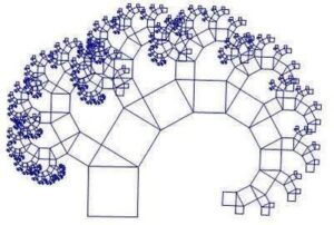
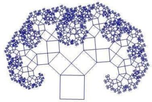
Dan Kennedy ‘s “Climbing around on the Tree of Mathematics,” (full text here) and Greg McColm’s “A Metaphor for Mathematics Education” are two recent articles that make arguments by analogy about what mathematics is and how it should be taught. In Kennedy’s argument, mathematics is a tree, while in McColm’s it is a vine – both are organic, growing, and branching. What distinguishes these two uses of metaphor from traditional tree analogies is that both authors are not at all suggesting that we can stand back and survey the structure as a whole and understand how all its parts are related. The ability to provide a comprehensive view of the subject, to make it surveyable, was the raison-d’être of metaphors like the “Tree of Science.” Instead of using the metaphor this way, both authors suggest that we think of ourselves as part of the growing structure – as climbers and gardeners who cannot see the complex organic whole, but who can explore and tend to our small part of it. In these descriptions, natural forms like trees and plants, once metaphors for simplicity and comprehensibility, now provide metaphors for complexity.

Up in the Tree of Mathematics, Kennedy suggests that working mathematicians are labouring at extending its outer branches. This is where the view is best, where the fruit is found, and where the beauty of mathematics can be seen most clearly. School Mathematics is part of the trunk, the solid, oldest, stable part of the tree, and math teachers spend their time helping students climb the trunk, hoping that some may one day reach its outer branches. Unfortunately, the difficulty of the trunk prevents most people from ever climbing beyond it. Kennedy suggests that we should be less concerned with the trunk than with the branches, and that technology can provide a ladder to assist the climb.

McColm’s Mathematical Vine is not mathematics itself, but a structure that clings to the underlying reality of mathematical truth. Mathematics, in this analogy, is like a hidden tower, whose shape can only be seen by looking at the vine that has taken shape around it. Like in Kennedy’s analogy, working mathematicians are the caretakers who help the structure grow. For McColm, this analogy emphasizes the importance of mathematics education – a process of strengthening the vine so that it may continue to grow. Perhaps because his audience is primarily post-secondary researchers, he does not advocate finding shortcuts to “higher” views, but rather suggests that education be promoted through “tending to the vine” – clarifying mathematics and strengthening connections between different branches.

Although they suggest more of a structure at play, rather that a stable unified whole, organic metaphors like those used by McColm and Kennedy continue to suggest a natural unity among the various parts of mathematics. In that sense they are still rooted (or centered), and, although they have somewhat destabilized the tree analogy, they haven’t quite deconstructed it. They have not, for example, gone quite as far as Wittgenstein, who seemed to suggest that metaphors that attempt to link the subjects of mathematics in a defining way like this are misguided. In his view, as described by Ackerman (1988, p. 115):

mathematics is an assemblage of language games, having no sharp and uniform external boundary, with potentially confusing and criss-crossing subdisciplines held together by an internal network of analogous proof techniques.

It is easy to appreciate how some climbers in Kennedy’s trees and McColm’s vines end up like the protagonist in Roz Chast’s cartoon “Falling off the Math Cliff”, where step 1 is “A boy begins his wondrous journey,” and step 8 is “The plummet.”

The images in this post are “Pythagoras Tree” fractals, made using GSP.

For more such insights, log into www.international-maths-challenge.com.

*Credit for article given to dan.mackinnon*

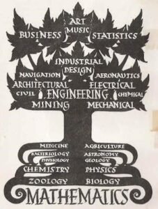
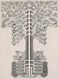
When asked to describe mathematics we often resort to metaphor rather than attempt to provide strict definitions. These pictures from high school math textbooks from the 1930s are an example of this tendancy.

The simple hierarchies of these images resolve the complicated relationship between mathematics and science by appealing to our desire for an organic unity among disciplines, giving mathematics a foundational role within the general concept of science. These images are appealing, but do not stand up to scrutiny.

The simple relationship between mathematics and science becomes complicated when mathematics is described, as it sometimes is, as a science itself. It’s definition as “the science of space and quantity” is further complicated by the caveat that it is an exact deductive science, unlike the usual inductive kind. Following this line of thinking further, mathematics is then described as a kind of meta-science, or a limit point to which science might aspire – science emptied of all of its empirical content, a science of pure thought. While some view mathematics as a foundation for science, others as a supra-science, the emerging field of experimental mathematics brings mathematics back into the empirical fold, reducing it (or elevating it) to a science like any other. So, mathematics can be seen as root, branch, or even the form of the tree itself.

Thinking about these things for even a short while evokes some sympathy with Bertrand Russell’s remark that “mathematics may be defined as the subject in which we never know what we are talking about, nor whether what we are saying is true.”

For more such insights, log into www.international-maths-challenge.com.

*Credit for article given to dan.mackinnon*

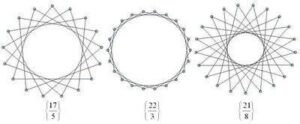
Starting with p (p a positive integer) equally distributed dots (vertices) around a circle. Connecting each dot to the next as you move around the circle will give you a regular p-gon – a p-sided polygon with p vertices. If, however, instead of connecting each dot to the one next to it you skip over a fixed number of dots, then you might end up with a star-like pattern, like the ones shown above. In this process, imagine that you start with a particular vertex and move in a counter-clockwise direction. If there are any dots left-over when you get back to the dot you started from, just throw away the unconnected dots.

The Schläfli notation for polygons is very useful for describing regular connected star polygons, and provides an example of how sometimes calculations with notation match exactly with calculations done with diagrams. In this notation, regular polygons like triangle, square, pentagon, etc. are written as {3}, {4}, and {5} respectively. A regular p-gon is written as {p}. If when drawing your p-gon you connect to the second next vertex instead of the first, then you would write this as {p/2}. If you connect to the q’th next vertex, then you would write this polygon as {p/q}. Note that if you are just connecting to the next vertex to make a regular p-gon, this notation gives you {p/1} = {p}, as you would expect.

If you start playing with this process you will notice that {p/q} gives you the same polygon as {p/(p–q)} (as long as you ignore the orientation of the polygon). You may also notice that if q is larger than p, you end up repeating the same patterns, in particular {p/q} = {p/(q mod p)}. Also you will notice that if p and q have common factors, you end up having skipped vertices. In our process we are throwing these away to ensure that our polygons are connected, but you can extend the process and keep them (see note below).

The process described is straightforward to implement in a program. The images shown here were generated in Tinkerplots. To implement it in Tinkerplots, you need two sliders – p and q, and the following attributes:

n = caseIndex()
theta = 2*n*pi(1-q/p)
x = cos(theta)
y = sin(theta)

If you create a plot with y vertical and x horizontal, choose “show connecting lines” and add a filter n<=p+1, you can add a large number of cases to the collection (~200, say) and be able to slide p and q to create a wide variety of connected star polygons. The only restriction is that p must be less than the number of cases you have created. There is nothing special about using Tinkerplots here – any programming environment with reasonable graphics should do a reasonable job (Logo would be fine. :)).

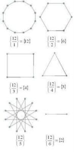
The polygons below are the regular connected polygons based on 12 vertices. Because 12 is divisible by 2, 3, 4, and 6 we end up with regular polygons triangle {3}, square {4}, hexagon {6} and only one star polygon {12/5}. The “degenerate” polygon {2} is known as a “digon.” Here, drawing the diagram first and then seeing what polygon comes out will give you the same result as dividing p/q first and then drawing the corresponding polygon. In this sense, the notation and diagrams nicely reflect each other.

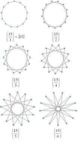
Contrast this with the family of star polygons that are generated when a prime number of vertices are used. The images below are the family of regular connected polygons generated on 13 vertices.

Note – by throwing away the unconnected dots in our process we are ignoring star polygons that are made of overlapping disjoint star or regular polygons, for example two overlapping triangles that make a star of David. These also work well with the Schläfli notation. To create these overlapping polygons, if you have any skipped vertices, you just begin your process again beginning with one of the vertices you skipped over. In the case of {6/2}, instead of getting one triangle {3} you will get two overlapping triangles, or 2{3}. To write a program that would draw these you would want to use something more sophisticated than Tinkerplots.

For more such insights, log into www.international-maths-challenge.com.

*Credit for article given to dan.mackinnon*

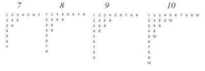
A surprisingly interesting structure is the extended multiplication table, shown above for the numbers seven to ten. The algorithm for drawing these is straight forward – for an n-extended table, start out as if you were writing a “regular” multiplication table, but extend each row so that it gets as close to, without exceeding, n. Another way to think about it is to write out rows of “skip counting up to n” by i for integers i from 1 to n.

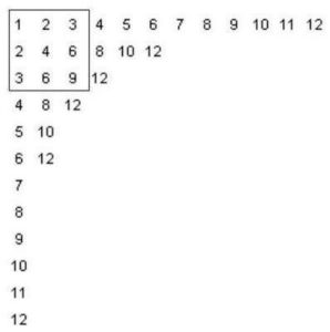
This is called an extended multiplication table since it contains a “traditional” multiplication table inside it. The 12-extended table below contains a traditional 3×3 multiplication table.

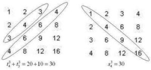
It turns out that 1 appears in an extended table once, and prime numbers appear exactly twice (once in the first column, and once in the first row). In general, for a natural number n, how many times does n appear in the n-extended table?

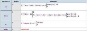
Before looking at that question, you might want to think about finding easier ways to draw the tables. Drawing out these tables by hand can be tedious – a simple program or spreadsheet might be easier. You can use Fathom, for example, to create the table data and draw it in the collections display. Create a slider m and the attributes listed in the table below (click on the image to see a larger version).

Modify the collection display attributes to draw the tables in the collection box. By adding lots of cases and using the slider m to filter out the ones you don’t need, you can vary the size of the table easily.

“how many times does n appear in the n-extended table?”

# of occurrances of n in the n-extended table = # of nodes in the factor lattice Fn

You can also recast both of these questions (how many occurances of n in the n-extended table, and how many nodesin the Fn factor lattice) as a combinatorial “balls in urns” problem.

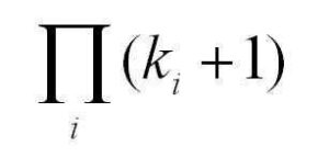
Consider a set of colored balls where there are m different colours, where there are ki balls of color i, where i ranges from 1 to m. This would give a total number of balls equal to k1+k2+…+km. Suppose you were to distribute these balls in two urns. How many different distributions would there be? Using some counting techniques, you will find that the answer is (k1+1)*(k2+1)*…*(km+1).

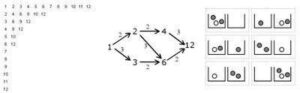
How is this connected to the other problems? Consider the prime factorization of the number. For each prime, choose a colour, and for each occurance of the prime in the factorization, add a new ball of that color. For example for 12 = 3*3*2, choose two colours – say blue=3 and red=2. Since 3 occurs twice and 2 occurs once, there should be two blue balls and one red ball. Now consider distributing these balls in two urns. It turns out that you get (2+1)*(1+1) = 6 possibilities. This is the same number of times 12 occurs in the 12-extended table, and the same number of nodes in the 12-factor lattice. The image below shows the 12-extended table, the 12-factor lattice, and the “ball and urn problem” for the numer 12.

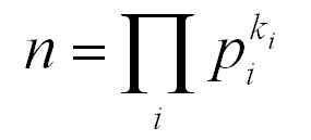
For a number n with the prime factorization:

The answer to all three questions is given by:

For more such insights, log into www.international-maths-challenge.com.

*Credit for article given to dan.mackinnon*

Robert Recorde, author the first English textbook on algebra (published in 1557), chose to give his book the metaphorical title The Whetstone of Witte to encourage people to take up the new and difficult practice of algebra. The metaphor of a whetstone, or blade-sharpener, suggests that algebra is not only useful, but also good mental exercise. In the verse that he included on its title page, he writes,

Its use is great, and more than one. Here if you lift your wits to wet, Much sharpness thereby shall you get. Dull wits hereby do greatly mend, Sharp wits are fined to their full end.

Mathematics, and algebra in particular, according to The Whetstone of Witte is like a knife-sharpener for the brain. Four hundred years later, in his book Mathematician’s Delight (1961), W.W. Sawyer takes up a similar metaphor, suggesting that “Mathematics is like a chest of tools: before studying the tools in detail, a good workman should know the object of each, when it is used, how it is used.” Whether they describe mathematics as a sharpener or other tool, these mechanical metaphors are commonly used to emphasize the practicality and versatility of mathematics, particularly when employed in engineering or science, and suggest that it should be used thoughtfully, and with precision.

An often quoted mechanical metaphor that suggests a more frantic and less precise process of mathematical creation is often attributed to Paul Erdos: “a mathematician is a machine for turning coffee into theorems.”

For more such insights, log into www.international-maths-challenge.com.

*Credit for article given to dan.mackinnon*

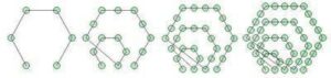
Polygonal numbers are a mainstay of recreational and school mathematics, providing a nice bridge between numbers and shapes. The diagrams above show some of the hexagonal numbers.

Some examples of two-dimensional polygonal numbers are:

the triangular numbers: 1, 3, 6, 10, 15, …
the square numbers: 1, 4, 9, 16, 25, …
the pentagonal numbers: 1, 5, 12, 22, 35,…
the hexagonal numbers: 1, 6, 15, 28, 45, …

Comparing the listing for the hexagonal numbers with the diagrams above, you can see how the sequences are built diagrammatically. In general, beginning with a single dot, k-sided polygons are built by adding layers (called gnomons) consisting of k-2 segments, with each segment of the gnomon having one more dot than the segments of the previous layer. In this way, the nth gnomon consists of segments each n dots long, but with k-3 dots shared by adjoining segments (the corners).

The description above can lead you to a recursive formula for k-polygonals, writing p_k,n for the nth k-polygonal number:

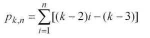
Unwinding the recursion gives you a summation formula for k-polygonals:

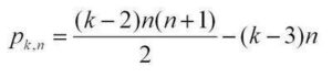
Knowing a little about sums gives you the direct formula for k-polygonals:

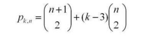
Coming a little out of left-field is this combinatorial formula for k-polygonals:

This last formula expresses two ideas: that the triangular numbers correspond to the r=0 column of Pascal’s triangle, and that every polygonal number can be “triangulated”:

The combinatorial formula for p_kn can be generalized to higher-dimensional polygonal numbers (pyrimidal numbers, etc.).

The recreation here lies in showing that the various formulas for p_k,n are really the same, and then exploring the relationships between the different k-polygonals. A great resource is J.H. Conway and R.K. Guy’s The Book of Numbers.a

For more such insights, log into www.international-maths-challenge.com.

*Credit for article given to dan.mackinnon*

Looking at the last few digits that appear in the numbers that form the sequence b^0, b^1, b^2, b^3, … for b a positive integer, you’ll notice that the digits will always begin to repeat after a certain point. For example, looking at the last digit of the sequences for b = 2, 3, and 4 we have the sequences

b = 2: 1, 2, 4, 8, 6, 2, 4, 8, 6, …
b = 3: 1, 3, 9, 7, 1, 3, 9, 7, …
b = 4: 1, 4, 6, 4, 6, 4, 6, …

If we look at the sequence of last two digits of these sequence where b =2 we have

b = 2: 1, 2, 4, 8, 16, 32, 64, 28, 56, 12, 24, 48, 96, 92, 84, 68, 36, 72, 44, 88, 76, 52, 4, …

This sequence then repeats the loop that began at 4.

We can describe these sequences as T_b,d(n) = (b^n)mod 10^d. Recursively, T_b,d(n) = (T_b,d(n-1)*b)mod 10^d

These sequences are always eventually periodic. Although these sequences are simple to understand and calculate, there are several interesting ways of describing them.

For example, you can think of the elements of T_b,d as a commutative monoid, with multiplication defined as a*b = (a*b)mod 10^d. They form a monoid since 1 is always a member, and you can show that T_b,d is closed under the * operation. It turns out that for some values of b, and d, T_b,d is a group.

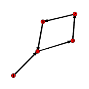
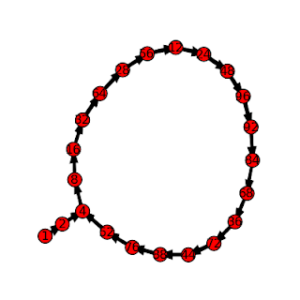
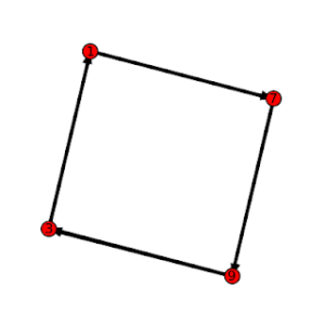
You can also think of this set as a finite state machine or graph, where each element is a node and the transition from one node to the next is defined by the operation *b mod 10^d. This provides a nice way of displaying the sequences. The pictures in this post were created by writing a short program to calculate the sequences, and then formatting the output to draw a di-graph in SAGE. The graph at the top of the post is for b=8, d=1, while the graph below is for b=2, d=2. The graph at the bottom of the page is for b=7, d=1.

For more such insights, log into www.international-maths-challenge.com.

*Credit for article given to dan.mackinnon*

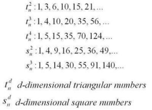
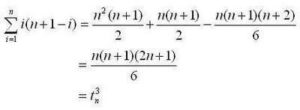
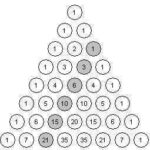
The third diagonal column in Pascal’s Triangle (r = 2 in the usual way of labeling and numbering) consists of the triangular numbers (1, 3, 6, 10, …) – numbers that can be arranged in 2-dimensional triangular patterns. The fourth column of Pascal’s triangle gives us triangular-based pyramidal numbers (1, 4, 10, 20, …), built by stacking the triangular numbers. The columns further out give “higher dimensional” triangular numbers that arise from stacking the triangular numbers from the previous dimension.

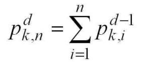
It is not by coincidence that the triangular and higher-dimensional triangular numbers appear in Pascal’s Triangle. If you think about layering of polygonal numbers in terms of equations, you get

In the above equation p^d_(k,n) is the nth k-polygonal number of dimension d. Triangular numbers are the 3-polygonal numbers of dimension 2, square numbers are the 4-polygonal numbers of dimension 2, “square based pyramidal numbers” would be denoted as p^3_(4,n).
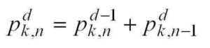
from the sum above, you can obtain this equation:

Which looks very much like the Pascal Identity C(n,r) = C(n-1,r-1) + C(n-1,r), except for some translation of the variables. To be precise, if we consider the case where k=3 and use r = d and n‘ = n+d-1 we can translate the triangular numbers into the appropriate positions in Pascal’s Triangle.

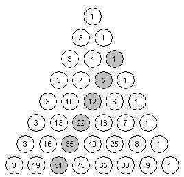
Along with the definitions for the end columns, the Pascal Identity allows us to generate the whole triangle. This suggests the following strategy for calculating the higher k-Polygonal numbers: create a modified Pascal’s Triangle whose first column is equal to k-2 (instead of 1), and whose last column is equal to 1 (as usual). This modified Pascal’s Triangle is generated using these initial values and the usual Pascal Identity.

Here is an example with k=5, which sets the first column values equal to 3 (except for the top value, which we keep as 1) and yields the pentagonal numbers (column 3) and the higher pentagonal numbers.

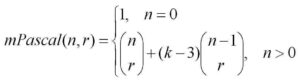
The formula for these modified Pascal Triangles is given by this equation:

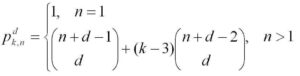
If we apply the change of variables mentioned above, we can obtain this general formula for the higher polygonal numbers in terms of combinations:

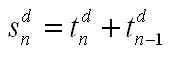
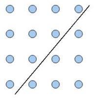
This formula illustrates how polygonal numbers are built out of triangular numbers. It says that the nth d-dimensional k-polygonal number is equal to the nth d-dimensional triangular number, plus (k-3) copies of the n-1 d-dimensional triangular number. This is a little easier to understand when you forget about the higher-dimensions and look at the regular 2-dimensional polygonal number.

For more such insights, log into www.international-maths-challenge.com.

*Credit for article given to dan.mackinnon*

John Sims has created a number of pi-related art works. One, the Pi Color Map, can be recreated effectively using TinkerPlots. The image above is one such Pi Color Map, using 2281 digits of pi.

Here are some instructions for creating a Pi Color Map in Tinkerplots.

1. Obtain a listing of the digits of pi – up to a reasonable number. You can get the digits from several sites, including the pi day site.

2. Paste your listing to a text document, and get them arranged into a single column. One strategy for doing this is and use the find/replace feature of a word-processor to replace each number with the number itself plus a line-break(e.g. in Word, replace 2 with 2^l, etc.).

3. If you’ve included the decimal point, remove it. For the first line of your document, provide a heading like pi_expansion. This will be your TinkerPlots attribute.

3. Import the text file into TinkerPlots using the File>Import menu.

4. Create a new attribute called digit whose formula is digit=concat(“”,pi_expansion). This creates a categorical data type that TinkerPlots won’t treat numerically. This is what you will use as your color key. Using the pi_expansion attribute gives a spectrum of color, rather than distinct colors for each number.

5. Create a new attribute called place, whose formula is place=caseIndex. This is what you will order your plot by.

6. Create a new plot, lock the color key on the digit attribute. Select the place attribute and press the Order By button.

7. Change your icon type to small squares, and stack the cases.

You can play with different options to get different effects for your color map.

One nice thing about doing this in TinkerPlots is that you can investigate the data further. The color map plot highlights the apparent randomness of the pi expansion, but you can also create other attributes and plots to investigate things like the running average of the digits, occurrences of consecutive digits, and the overall distribution of the digits (it should be uniform).

For more such insights, log into www.international-maths-challenge.com.

*Credit for article given to dan.mackinnon*

If You take a look at the square numbers (n^2, n a positive integer), you’ll notice plenty of patterns in the digits. For example, if you look at just the last digit of each square, you’ll observe the repeating pattern 1, 4, 9, 6, 5, 6, 9, 4, 1, 0, … If you construct a graph of “last digit” vs n (like the one below, built with Falthom), the symmetry and period of this digit pattern is apparent.

Why does this happen? The periodic nature of the pattern is easy to understand – when you square a number, only the digit in the ones place contributes to ones place of the product. For example, 22*22 and 32*32 are both going to have a 4 as their last digit – the values in the tens place (or any other place other than the ones) do not affect what ends up as the last digit.

The reason for the symmetry about n=5 is a little less obvious. To see what is going on, it is helpful to use modular arithmetic and to realize that ” last digit of n” is the same as “n mod 10”. Considering what 10-n looks like mod 10 after it is squared, we have the equation below.

This tells us that the last digit of (10-n)^2 is the same as the last digit of n^2, because everything else that is different about these two numbers is divisible by 10.

If you look at the last two digits of the square numbers, you see another repeating pattern that has similar symmetries.

This is a nice looking graph – the period is 50 with a line of symmetry at n=25. You can think about it in the same way as the one-digit case, this time the symmetry is understood by looking at (50-n)^2 mod 100. (Looking at numbers mod 100 tells us their last two digits.)

If you decide to investigate patterns in cubes or higher powers, you’ll see somewhat similar results. Using the binomial theorem and modular arithmetic, you can see why even powers give symmetry similar to the n^2 case, while odd powers do not (although all are periodic).

This graph shows the pattern in the last digit of n^3.

This last graph shows the pattern for the last two digits of n^4.

For more such insights, log into www.international-maths-challenge.com.

*Credit for article given to dan.mackinnon*