Category: mathematics

With connections to the study of gambling, Brownian motion, fractals, and more, random walks are a favourite topic in recreational mathematics.

The diagram above (from Energy transformations during horizontal walking by F. G. Benedict and H. Murschhauser, published in 1915) suggests one method for generating walking data. Creating random walk simulations in Fathom or TinkerPlots is a little more straightforward.

First simulation – using sliders to determine a ‘base angle’

This first example lets you set up random walks where the direction chosen is based on an angle k*2pi/n for a fixed n (whose value is determined by a slider) and a random k (a random integer between 1 and n).

First, create a slider n, then create the attributes below and finally add the data (any number is fine – start with ~500 cases). The formulas below were entered in TinkerPlots, but would work equally well in Fathom.

Plots of (x,y) will show the walk, and plots of (step, distance) will show how the distance from the origin changes over the course of the walk. Different values for n provide walks with their own particular geometries.

The walks start at (0,0) and wander about the plane from there. Re-randomizing (CNTRL-Y) generates new walks.

The simulation gives lots of nice pictures of random walks. You could generate statistics from these by adding measures and measure collections.

One limitation of this simulation is that it is difficult to determine exactly when the walker has returned to the start (0,0).  This turns out to be an interesting question for random walks on the plane (see the wikipedia entry for more on this). Because of the inexactness in the positions calculated using sine and cosine, the walker seems to never return to the origin. There are several ways of dealing with this, but one is to design a simpler simulation that uses exact values – one that sticks to lattice points (x, y), where x and y are both integers.

Second simulation – sticking to Integer lattice points

This second simulation can be thought of an ‘urban walker’ where all paths must follow a strictly laid out grid, like some downtown streets. The exactness of the positions means that we can detect with confidence when the walker has crossed back to their starting point. For this simulation, no slider is required – just enter the attributes and add cases.

Using the crossed_start attribute as a filter or to gather measures, you will find that walks often quickly pass over the starting point. You will also find that as you increase the number of cases, the straight ‘etch-a-sketch’ lines of the urban walk take on very interesting fractal-like contours.

For more such insights, log into www.international-maths-challenge.com.

*Credit for article given to dan.mackinnon*

It could be argued that the square is the ‘nicest’ rhombus, but the rhombus with angles of 60 and 120 degrees seems nicer still. One of the nice things about the 60/120 rhomb are the plane tilings that can be constructed from it. One of these tilings is the ‘tumbling blocks’ tiling shown at the top of the post, in which at some points you see ‘cubes’ (around the degree 3 vertices), while at others you see ‘flowers’ (around the degree 6 vertices). Because of the two different types of vertices, this is known as a quasi-regular rhombic tiling. (Another tiling that uses the 60/120 rhomb is this one.)

If you want to build a polyhedron that resembles the tumbling block tiling, one method is to reduce the number of petals in your flowers to 5, and then stretch your 60/120 rhombs until they are have angles of 63.435 and 116.565 degrees. Thirty of these rhombs arranged around vertices of degree 3 and 5 produces a quasi-regular polygon known as the rhombic triacontahedron.

The image above is of a model that was built using rhombic units printed onto card stock.

Despite the apparent ugliness of the 63.435 and 116.565 degree angle-measurements, our nice 60/120 rhomb has been, arguably, stretched into an even nicer one – a ‘golden rhombus,’ so called because the ratio of the diagonals is equal to the golden ratio.

The dual of the rhombic triacontahedron is the archemedian polyhedron known as the icosidodecahedron.

For more such insights, log into www.international-maths-challenge.com.

*Credit for article given to dan.mackinnon*

Imagine a tetrahedron centered inside a sphere. If you were to project the edges of the tetrahedron out from the center so that they touched the surface of the sphere, the edges would cut the sphere in arcs that lie on the sphere’s ‘great circles’ (the largest possible circles drawn on the surface of the sphere – circles whose radii are the same as the radius of the sphere).

The image at the top of this post shows a model of a sphere with the six great circles formed by the projected edges of a tetrahedron sitting at its center.

The model, described on pages 4 and 5 of Magnus Wennigers’ Polyhedron Models, is easy to construct using the template shown below. Printing copies of the template onto card-stock and gluing them together works well. This pdf file has 10 arcs on a single page for printing (you will need 24 arcs in total).

Each arc is folded and glued to form a spherical triangle, 24 of the spherical triangles glued together will form the sphere.

The diagram below (based on Fig.2, p.5, in Wenniger) shows how to assemble 6 of the triangles into one ‘face’ of the spherical tetrahedron. Four of the faces can be assembled into the ‘spherical tetrahedron.’ When assembling, you should make sure that you align the triangles so that they form great circles.

Spherical triangles, as you can tell from the diagram, do not follow the rule of having their interior angles sum to pi (180 degrees), as plane triangles do.

The arc is divided into angles of 54deg&44min, 70deg&32min, 54deg&44min, as described by Wenniger. The template was created in GSP.

For more such insights, log into www.international-maths-challenge.com.

*Credit for article given to dan.mackinnon*

There are plenty of probability problems that have counter-intuitive solutions. Problems like these, and how they can undermine common sense, are among the best reasons for looking at probability theory. One set of humbling questions is the family of Monty Hall problems. Another are those related to conditional probability; nice examples of these are problems that involve medical tests that give ‘false positive’ results.

Simulation is a way of exploring these problems that reveals more than mere theoretical probability calculations do. The structure of the simulation can reflect interesting aspects of the structure of the original problem, and the results reveal a variability that is not apparent when you simply calculate the theoretical probabilities on their own.

This post shows an example of a ‘false positive’ probability problem and a Fathom simulation for it. This problem was adapted from one found in the 4th edition of Ross’s A First Course in Probability (p.75):

A laboratory blood test is 95 percent effective in detecting a certain disease when it is, in fact, present. However, the test also yields a “false positive” result for one percent of healthy persons. (That is, if a healthy person is tested, there is a 0.01 probability that they will test positive for the disease, even though they don’t really have it.) If 0.5 percent of the population actually has the disease, what is the probability that a person who has a positive test result actually has the disease?

Here are the attribute definitions that you could use to build a Fathom simulation for this problem:

The attributes are enough to run the simulation, but it is better to also add the following measures:

To run the simulation you can add new cases (try ~500). Using a measures collection, you can re-run this experiment hundreds of times (collecting a 100 measures re-runs the 500 person experiment 100 times).

If you are calculating the theoretical probability by hand, it helps to write down all of the probabilities (fill in the blanks…):

It also helps to visualize the probabilities in a tree diagram:

The outer tips of the tree are filled in using the multiplicative rule for conditional probabilities:

One nice thing about doing this is that you can see how the tree diagram used to calculate the theoretical probabilities is structured in the same way as the “if” statements in the simulation.

For more such insights, log into www.international-maths-challenge.com.

*Credit for article given to dan.mackinnon*

Students generally learn to divide polynomials using  long division or synthetic division. This post is about another method for dividing polynomials,  the “grid” method. Although this method is used at some schools, I have not found it in any textbook (if you know of any, please let me know).

The grid method makes polynomial division a fun calculation – an almost SUDOKU-like process. The recreational challenge here is to master the method, and to convince yourself that it actually works in all cases (which cases does it work well for, and which are more difficult?).

Before tackling polynomial grid division, you need to be familiar with polynomial grid multiplication. It is the symbolic analog to the familiar “algebra tiles” manipulative, so if you have worked with these, it should be reasonably familiar.

Polynomial Grid Multiplication

In polynomial grid multiplication, the two factors are arranged on the edges of a grid – the number of terms of the factors determine the number of horizontal and vertical lines that make up the grid.

The overall product is found by filling in the cells of the grid with the product of the terms for the row and column, and then summing up all the contents of the interior of the grid.

What polynomial grid multiplication does for us is provide an explicit way to keep track of the distributive property: each term-by-term product gets its own cell.

In the example below, the two factors are placed along the edges of the grid (1). One factor provides the row headings, the other provides the column headings. Then each cell is filled in with the product of the terms from the row and column (2). Finally, the cells are added together (like terms are combined) to find the final product (3). If the terms of the factors are placed according to the same order (descending powers of x, in our example) and there are no missing terms, then like-terms of the product are found along the diagonals of the grid.

Polynomial Grid Division

Polynomial grid division works the same way as polynomial grid multiplication, but in reverse – we start by knowing one of the factors (placed along the edge of the grid), and by knowing what we want the product to be (without knowing exactly how it is ‘split up’ in the grid). Using this knowledge we work backwards, filling in the grid and the top edge one cell at a time until we are done.

Consider the example below. In (1) we create an empty grid with the denominator (divisor) playing the role of one of the factors. Since this question involves a degree 3 polynomial divided by a degree 1 polynomial, we know that the other factor (the quotient) must be degree 2. This allows us to create a grid with the correct size. In step (2) we use the highest power of the dividend (the numerator) to begin to fill in the grid – we know that 27x^3 must be in the top left. This in turn tells us that the first column entry must be 9x^2 (so that the row and column multiply to 27x^3). In step (3) we use this to fill in all of the first column, multiplying 9x^2 by the terms of the row entries.

In step (3) we now have a quadratic term -18x^2. But we know from looking at the dividend (numerator) that in the final answer we actually want 9x^2. Consequently, the other entry on the quadratic diagonal must be 27x^2, so that the whole diagonal sums to 9x^2 .  Filling this in for step (4) tells us what all the entries in the second column should be (step 5). Now that we have a linear entry -18x, we know that we need to add in a 15x so that the overall sum gives a -3x (step 6).

Having a 15x tells us that the top entry must be 5 (the product of 5 and 3x gives us 15x). Filling this in in step 7 allows us to complete the table, and we see that our final constant entry is -10, as hoped for. Now that the grid has been filled in and it matches the dividend, we can read the answer off the top – the factor that we have uncovered is the quotient we were hoping to calculate.

This method is actually easier than it seems at first, and when all steps are carried out on the same grid, is quite compact.

Here is another example for you to try it out on.

In these two examples, the division worked well – there was no remainder. In the case where we are dividing f/g and g is not a factor of f, and the degree of g is less than the degree of f, there is polynomial remainder whose degree is strictly less than that of g. So, for example, when g is a linear function (degree 1), f/g can have a constant remainder (degree 0).

In this case we proceed as above, attempting to fill in the grid with the numerator (dividend). However, if when we are done the grid does not match the numerator, we have a remainder. The remainder is the additional amount that we have to add to the grid in order to arrive at the numerator.

Consider a division question almost identical to the first one that we looked at, except here we change the numerator slightly so that it doesn’t factor well.

Following the same steps as before, we end up with a grid sum that does not match our desired answer: we have -10 instead of -9 for the final constant term. This tells us that we have a remainder of +1, that we choose to write next to the grid. In our final answer, the remainder tells us the “remaining fractional part” that we have to add at the end.

For more such insights, log into www.international-maths-challenge.com.

*Credit for article given to dan.mackinnon*

Here is an outline of how you can go about generating this data. The definition and properties of Farey sequences here are from Hardy & Wright’s An Introduction to the Theory of Numbers (which I am slowly working my way through).
The Farey sequence of order n is the sequence of irreducible fractions between 0 and 1 whose denominator does not exceed n. So, the elements of the sequence are of the form h/k, where h < k < n, and h and k are relatively prime.

The main theorem about Farey numbers provides them with their characteristic property (Theorem 29 in TofN). The characteristic property of Farey sequences is that if h/k, h”/k”, and h’/k’ are successive terms in a Farey sequence, then h”/k” is the mediant of h/k and h’/k’. If h/k and h’/k’ are two reduced fractions, their mediant is given by (h+h’)/(k+k’).

It’s nice when a theorem tells you how to implement an algorithm. This property tells us that Farey sequences can be built iteratively or recursively, beginning with F1={0/1 ,1/1}. The algorithm to do this is a nice one – it’s probably not often used as a textbook exercise in recursion because it helps if you to have some data structure or class to represent the fraction, and a way of telling if integers are relatively prime (you can use the Euclidean algorithm to implement a gcd() function).

Here is an outline of how to calculate the next Farey sequence, given that you have one already.

0) input a Farey sequence oldSequence (initial sequence will be {0/1, 1/1})

1) create a new empty sequence newSequence

2) iterate over oldSequence and find out its level by finding the largest denominator that occurs store this in n

3) set n= n+1

4) iterate over oldSequence, looking at each pair of adjacent elements (left and right)

4.1) add left to newSequence
4.2) if the denominators of left and right sum to n, form their mediant
4.2.1) if the numerator and denominator of the mediant are relatively prime, add mediant to newSequence

5) add the last element of oldSequence to newSequence

Note that you only need to add in new elements where the denominators of existing adjacent elements sum to the n value – when this happens you form the mediant of the two adjacent elements. Furthermore, the mediant is only added if the fraction can’t be reduced.

Below is some Java-ish code corresponding to the above – it assumes that the oldSequence and newSequence are an ArrayList and that you have a class Fraction that has fields num (numerator) and den (denominator).

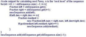
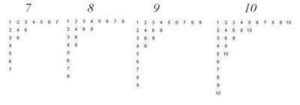
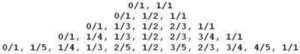
Here are the first five Farey sequences that you get from the algorithm:

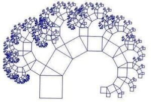
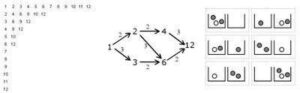
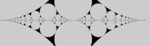
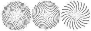
The image at the top of the post was generated by implementing the algorithm in Processing, and using the result to draw the associated Ford circles – you could do something similar in regular Java (or other language). If you draw the Ford Circles associated with the sequence, the circle for a fraction “frac” will be centered at (x,y) and have a radius r where

x = (scale)*frac.num/frac.den

y = r

r = (scale)/(2*(frac.den)^2)

where “scale” is some scaling factor (probably in the 100’s) that increases the size of the image.

Here I decided to draw two copies of each circle, one on top of the other.

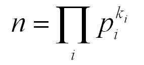
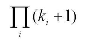
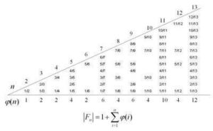
That it contains only fractions between 0 and 1 and that it contains all reduced fractions for denominators k < n, connects Farey sequences to Euler’s totient function. Euler’s totient function is an arithmetic function that for a given k, counts the integers less than k that are relatively prime to it. This is exactly the number of times that a fraction of the form h/k will appear in the Farey sequence for k>1.

The Farey algorithm, how to draw Ford circles, and the connection to Euler’s totient function are described nicely in J.H. Conway and R.K. Guy’s The Book of Numbers – a great companion to a book like TofN.

For more such insights, log into www.international-maths-challenge.com.

*Credit for article given to dan.mackinnon*

As I make my way through Hardy & Wright’s An Introduction to the Theory of Numbers,  I am hoping to work it into my recreational math pursuits – coming up with interesting (but not too heavy) activities that correspond roughly to the material in the text.

The first two chapters are on the sequence of primes. Here’s the activity: obtain a list of primes, import them into Fathom, and construct plots that explore pn and pi(n) and other aspects of the sequence that manifest themselves in the first couple of thousand terms.

In my Fathom experiment, I imported the first 2262 prime numbers.

If you import a sequential list of primes into Fathom (under the attribute prime) and add another attribute n=caseindex, you can create two nice plots. Plot A should have prime as the x axis and n  as the y axis. This shows the function pi(n). To this plot you should add the function y = x/ln(x) and visually compare the two curves. Plot B should have the x and y axis reversed. On this graph, plotting the function y = x*ln(x) shows how closely this approximation for pn (the nth prime) comes to the actual values.

You can add further attributes to look at the distance between primes dist=prime-prev(prime), and also the frequency of twin primes is_twin = (dist=2)or(next(dist)=2).

You can also add attributes to keep a running count of twin_primes, and to keep a running average of the twin_primes. The plot above shows how the ratio of tiwn primes diminishes as the number of primes increases. The plot at the top of the post suggests the distribution of primes and twin primes (in blue) in the numbers up to the 2262nd prime.

For more such insights, log into www.international-maths-challenge.com.

Credit for article given to dan.mackinnon*

If mathematics is a game, then playing some game is doing mathematics, and in that case why isn’t dancing mathematics too?

Ludwig Wittgenstein – Remarks on the Foundations of Mathematics

Mathematics is often described metaphorically – the  forms that these metaphors take include the organic, mechanical, classical, and post-modern, among countless others. Within these metaphors, mathematics may be a tool, or set of tools, a tree, part of a tree, a vine, a game, or set of games, and mathematicians in turn may be machines, game-players, artists, inventors, or explorers.

Despite the many metaphors used to describe mathematics, in popular discourse mathematics is often reduced to one of its parts, being metonymically described as merely about numbers, formulas, or some other limited aspect. Metaphor is a more complete substitution of ideas than metonymy – allowing us to link concepts that do not appear to have any direct relationship. Perhaps, metaphoric language that elevates and expands our ideas about mathematics is used by enthusiasts to counter the more limited and diminishing metonymic descriptions that are often encountered.

Attempts to describe and elevate mathematics through metaphor seem to fall short, however. Our usual way of thinking about things is to inquire about their meaning – a meaning that is assumed to lie beneath or beyond mere appearances. Metaphor generally relies on making connections between concepts on this deeper level. The sheer formalism of mathematics frustrates this usual way of thinking, and leaves us grasping for a meaning that is constantly evasive. The sheer number and variety of the  many metaphors for mathematics suggests that no single convincing one has yet been found. It may be that the repeated attempts to find such a unifying metaphor represents an ongoing and forever failing attempt to grapple with the purely formal character of mathematics; and it may be that the formal nature of mathematics will always shake off any metaphor that attempts to tie it down.

For more such insights, log into www.international-maths-challenge.com.

*Credit for article given to dan.mackinnon*

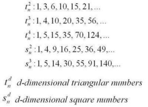
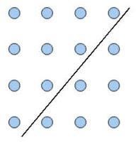
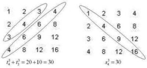
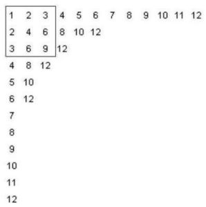
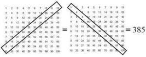A surprising relationship found in the multiplication table is that the sum of the entries in the main upwards diagonal and the diagonal above it is equal to the sum of the entries in the main downwards diagonal. What is also surprising is that this is but one among several observations about the multiplication table that can be expressed in terms of polygonal numbers.

This relationship involves three-dimensional triangular numbers (triangle-based pyramidal numbers, or tetrahedral numbers), and three-dimensional square numbers (square-based pyramidal numbers). Some values for these, and a few other polygonals, are shown below.

To see why this relationship holds, first note that the sum of the entries in the nth upward diagonal in the multiplication table is equal to the nth three-dimensional triangular number.

Second, observe that he entries in the main down diagonal are square numbers (two-dimensional), so the sum of the main down diagonal is the nth three-dimensional square number.

Finally, we use the fact that a square number (of any dimension) can be split into two triangular numbers (of the same dimension), which gives us the surprising result above.

the image below shows the relationship for a 4×4 multiplication table.

For more such insights, log into www.international-maths-challenge.com.

*Credit for article given to dan.mackinnon*

The names of the trigonometric ratios tangent and secant are derived from the Latin “to touch” and “to cut” – the tangent to a figure is a line that touches it in one place, where a secant cuts through it in two or more. But how are these geometric terms related to the ratios that bear their names? The answer can be shown using the diagram at the top of the post – a diagram that used to be a standard one in high school trig text books.

Consider the acute angle BAC. Allow |AC| = 1, and construct a unit circle about A that goes through C. Construct a tangent to this circle at C, and extend the segment AB so that it meets this tangent at E. So, the segment CE lies on the tangent while the segment AE lies on the secant of the unit circle formed around BAC. ACE is a new right triangle that contains the original BAC.

The tangent of BAC is BC/AB (opposite/adjacent), but if we now look at the second triangle ACE, we see tht it is also given by (CE/AC)=(CE/1)=CE – the tangent is measured by the segment of the tangent, CE. Similarly, the secant of BAC is given by AC/AB (hypoteneuse/adjacent), but again turning to the second triangle ACE, we see that this is (AC/AB)=(AE/AC)=(AE/1)=AE – and the secant is provided by the length of the secant, AE.

This treatment was taken from the book “Plane Trigonometry and Tables” by G. Wentworth, published in 1903. In some of the texts of this era, the “primary” trigonometric ratios were sin, sec, and tan (rather than sin, cos, and tan), perhaps owing their primacy to constructions like the one described above.

The cosine was considered a secondary trigonometric ratio – its name coming from the phrase “complement’s sine.” Along with the usual ratios, texts often presented several convienience ratios that are now antiquated, such as the versedsine vrsin(x) = 1-cos(x) and the half-versed sine or haversine hvrsn(x)= (1/2)vrsin(x).

The most fundamental trigonometric ratio has the most obscure name. It is generally claimed that the word “sine” comes from Latin word for “bend,” but some have suggested that the word is ultimately derived from the name of the curve formed by the gathering of a toga, or from the Latin word for “bowstring.” In Arithmetic, Algebra, Analysis, Felix Klein states that “sine” represents a Latin mis-translation of an Arabic word, but does not go on to explain its origins any further.

For more such insights, log into www.international-maths-challenge.com.

*Credit for article given to dan.mackinnon*