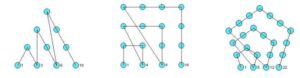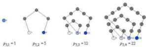
Drawing Polygonal Numbers

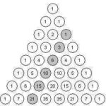
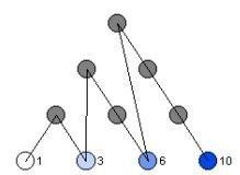
The diagram above (known as the tetractys) shows the first four triangular numbers (1, 3, 6, 10, …). Although there is a simple formula for calculating these numbers directly, t(n) = 1/2(n(n+1)), constructing them by these layered-triangle diagrams helps to show their geometric and recursive properties.

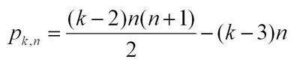
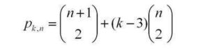
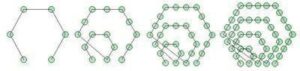
More generallypolygonal numbers arise from counting arrangements of dots in regular polygonal patterns. Larger polygons are built from smaller ones of the same type by adding additional layers of dots, called gnomons. Beginning with a single dot, k-sided polygons are built by adding gnomons consisting of k-2 segments, with each segment of the gnomon having one more dot than the segments of the previous layer. In this way, the nth gnomon consists of segments each n dots long, but with k-3 dots shared by adjoining segments (the corners).

This post describes how you can draw figures that illustrate the polygonal numbers and explore the polygonal numbers in general (triangular, square, pentagonal, hexagonal, etc.) using either TinkerPlots or Fathom. Both TinkerPlots and Fathom work well, but TinkerPlots creates nicer pictures, and allows for captions directly on the graph.
Without describing the details of how you create Fathom or TinkerPlot documents, here are the attributes that you will want to define in order to draw diagrams like the ones shown.

Required attributes
Create a slider k. This will allow you to set what kind of polygonal number you want to draw (k=3 gives triangular numbers, k=4 gives square numbers, etc.)
Define the following attributes:

The number itself. This is a natural number beginning at 1 and continuing through the number of cases.

gnomon This states which “layer” or gnomon the number belongs in. It is calculated based on a number of other attributes.

g_index This is the position of the number within the gnonom – it ranges from 1 up until the next k-polygonal number is hit.

s_index Each gonom is broken up into sections or sides – what is the position within the side? Each side is of length equal to the gonom number. The first gonom has sides of length 1, the second has length 2, etc.

corner This keeps track of whether or not the number is a “corner” or not. This is based primarily on the s_index attribute.

c_index This keeps track of how many corners we have so far. There are only k-1 corners in a gnomon (the first number n=1 is the remaining corner). So, when we hit the last corner, we know we are at a polygonal number.

k_poly Records whether or not the number n is k-polygonal. It does this by checking to see if it is the last corner of a gnonom.
The attributes listed above are required for finding the position of each number within the figure; th following attributes are used in actually drawing the figures.

angle The base corner angle for the polygon is determined by k. This is the external angle for each corner.

current_angle We have to add to the base angle at each corner as we turn at each corner. This attribute is used to keep track of the total current angle.

dx This is the x-component of the unit direction vector that we are travelling in. Each new dot moves one dx over in the x-direction. It is given by the cosine of the current angle.

dy This is the y-component of the unit direction vector that we are travelling in. Each new dot moves one dy over in the y-direction. It is given by the sine of the current angle.

prev_g_1_x This is the x-coordinate of the first dot in the previous gonom layer. We need to know this because it will be the starting point for the next layer – each layer starts back at the “beginning” of the figure.

prev_g_1_y This is the y- coordinate of the first dot in the previous gonom layer.

This is the x-coordinate of the current dot, calculated either from the previous dot or from the first dot in the previous layer.

y This is the y-coordinate of the current dot, calculated either from the previous dot or from the first dot in the previous layer.

caption Used to display the number on the plot (TinkerPlots only)
Below are the formulas for each attribute, written in “ascii” math. They are presented without a full explanation, in the hopes that if you try to implement this you will think about and explore each using the formulas and the descriptions above as a guide. Alternate methods for drawing the diagrams are possible, and you might find other formulas that achieve the same goals. Note that there are nested if() statements in several formulas.

n = caseIndex

gnomon = if(n=1){1, if(prev(k_poly)){prev(gnomon)+1, prev(gnomon)

g_index = if(n=1){ 1, if(prev(k_poly){1, prev(g_index) +1

s_index = if(n=1){ 1, if(prev(k_poly){1, if(prev(s_index) = gnomon){2,prev(s_index)

corner = (s_index=1) or (s_index=gnomon)

c_index= if(g_index=1){1, if(corner){prev(c_index)+1, prev(c_index)

k_poly = if(n=1){true, (c_index=k-1)

prev_g_1_x = if (n=1){0, if(g_index=2){prev(x), prev(prev_g_1_x)

prev_g_1_y = if(n=1){0, if(g_index=2){prev(y), prev(prev_g_1_y)

angle = pi-((k-2)*(pi/k))

current_angle = if(g_index =1) {pi-angle, if(pref(corner)){prev(current_angle)-angle, prev(current_angle)

dx = cos(current_angle)

dy = sin(current_angle)

x= if(n=1){0, if(g_index=1){prev_g_1_x +dx, prev(x) +dx

y =if(n=1){0, if(g_index=1){prev_g_1_y +dy, prev(y) +dy

caption = if(k_poly){n,””

To actually draw the diagrams, create a new plot with the x and y attributes as the horizontal and vertical axis, respectively. Add cases to the collection to populate the diagram. Optionally you can show connecting lines, and (in TinkerPlots) add a legend using the caption attribute.

For more such insights, log into www.international-maths-challenge.com.

*Credit for article given to dan.mackinnon*

This Turing Machine Should Run Forever Unless Maths is Wrong

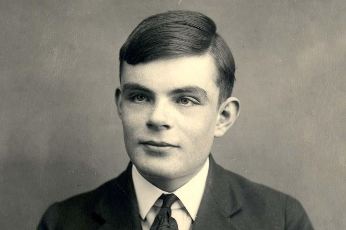
Alan Turing: still casting a long shadow over mathematics

One hundred and fifty years of mathematics will be proved wrong if a new computer program stops running. Thankfully, it’s unlikely to happen, but the code behind it is testing the limits of the mathematical realm.

The program is a simulated Turing machine, a mathematical model of computation created by codebreaker Alan Turing. In 1936, he showed that the actions of any computer algorithm can be mimicked by a simple machine that reads and writes 0s and 1s on an infinitely long tape by working through a set of states, or instructions. The more complex the algorithm, the more states the machine requires.

Now Scott Aaronson and Adam Yedidia of the Massachusetts Institute of Technology have created three Turing machines with behaviour that is entwined in deep questions of mathematics. This includes the proof of the 150-year-old Riemann hypothesis – thought to govern the patterns of prime numbers.

Turing’s machines have long been used to probe such questions. Their origins lie in a series of philosophical revelations that rocked the mathematical world in the 1930s. First, Kurt Gödel proved that some mathematical statements can never be proved true or false – they are undecidable. He essentially created a mathematical version of the sentence “This sentence is false”: a logical brain-twister that contradicts itself.

No proof of everything

Gödel’s assertion has a get-out clause. If you change the base assumptions on which proofs are built – the axioms – you can render a problem decidable. But that will still leave other problems that are undecidable. That means there are no axioms that let you prove everything.

Following Gödel’s arguments, Turing proved that there must be some Turing machines whose behaviour cannot be predicted under the standard axioms – known as Zermelo-Fraenkel set theory with the axiom of choice (C), or more snappily, ZFC – underpinning most of mathematics. But we didn’t know how complex they would have to be.

Now, Yedidia and Aaronson have created a Turing machine with 7918 states that has this property. And they’ve named it “Z”.

“We tried to make it concrete, and say how many states does it take before you get into this abyss of unprovability?” says Aaronson.

The pair simulated Z on a computer, but it is small enough that it could theoretically be built as a physical device, says Terence Tao of the University of California, Los Angeles. “If one were then to turn such a physical machine on, what we believe would happen would be that it would run indefinitely,” he says, assuming you ignore physical wear and tear or energy requirements.

No end in sight

Z is designed to loop through its 7918 instructions forever, but if it did eventually stop, it would prove ZFC inconsistent. Mathematicians wouldn’t be too panicked, though – they could simply shift to a slightly stronger set of axioms. Such axioms already exist, and could be used to prove the behaviour of Z, but there is little to be gained in doing so because there will always be a Turing machine to exceed any axiom.

“One can think of any given axiom system as being like a computer with a certain limited amount of memory or processing power,” says Tao. “One could switch to a computer with even more storage, but no matter how large an amount of storage space the computer has, there will still exist some tasks that are beyond its ability.”

But Aaronson and Yedidia have created two other machines that might give mathematicians more pause. These will stop only if two famous mathematical problems, long believed to be true, are actually false. These are Goldbach’s conjecture, which states that every even whole number greater than 2 is the sum of two prime numbers, and the Riemann hypothesis, which says that all prime numbers follow a certain pattern. The latter forms the basis for parts of modern number theory, and disproving it would be a major, if unlikely, upset.

Practical benefits

Practically, the pair have no intention of running their Turing machines indefinitely in an attempt to prove these problems wrong. It’s not a particularly efficient way to attack that problem, says Lance Fortnow of the Georgia Institute of Technology in Atlanta.

Expressing mathematical problems as Turing machines has a different practical benefit: it helps to work out how complex they are. The Goldbach machine has 4888 states, the Riemann one has 5372, while Z has 7918, suggesting the ZFC problem is the most complex of the three. “That would match most people’s intuitions about these sorts of things,” Aaronson says.

Yedidia has placed his code online, and mathematicians may now compete to reduce the size of these Turing machines, pushing them to the limit. Already a commenter on Aaronson’s SaiBlog claims to have created a 31-state Goldbach machine, although the pair have yet to verify this.

Fortnow says the actual size of the Turing machines are irrelevant. “The paper tells us that we can have very compressed descriptions that already go beyond the power of ZFC, but even if they were more compressed, it wouldn’t give us much pause about the foundations of math,” he says.

But Aaronson says shrinking Z further could say something interesting about the limits of the foundations of maths – something Gödel and Turing are likely to have wanted to know. “They might have said ‘that’s nice, but can you get 800 states? What about 80 states?’” Aaronson says. “I would like to know if there is a 10-state machine whose behaviour is independent of ZFC.”

For more such insights, log into www.international-maths-challenge.com.

*Credit for article given to Jacob Aron*


From English to Math

Let’s lay down some definitions:

  • Let FF be a field and let EE be an extension of FF. An element α∈Eα∈E is algebraicover FF if there is a polynomial f(x)f(x) in F[x]F[x] such that f(α)=0f(α)=0 (i.e. α∈Eα∈E is an algebraic element if it is the root of some polynomial with coefficients in FF).
  • Let FF be a field and let EE be an extension of FF. If K⊂EK⊂E is a subset of EE which contains all elements which are algebraic over FF, then KK is actually a subfieldof EE and an algebraic extension of FF. We call KK the algebraic closure of FF and denote it by ¯¯¯¯FF¯. [1]

It’s a fact that an algebraic closure ¯¯¯¯FF¯ exists for every field FF (and is actually unique up to isomorphism). So we can draw a containment picture like the one above.

Those familar with some topology and/or analysis will notice that such a “field tower” is suggestive of a vaguely analogous result: given a topological space XX we can always (assuming some conditions about XX, namely it being locally-compact Hausdorff) stick an open set VV and its closure ¯¯¯¯VV¯ between a certain compact set KK and open set UU:  K⊂V⊂¯¯¯¯V⊂U.K⊂V⊂V¯⊂U.

Now, don’t buy too much into the analogy. I only mention this topological result to motivate the fact that the closure of a set and the algebraic closure of a field do indeed convey the same concept: wholeness. It seems then that we can view algebraic elements as the mathematical cousins of limit points of sequences of real numbers. Why? Because, topologically speaking, what is the closure of a set? The collection of limit points of that set, right? So in particular, when we let our topological space be RR, the set of real numbers (with the usual topology) and consider the subset {xn}∞n=1{xn}n=1∞ – some sequence of real numbers,

  • we say x∈Rx∈R is a limit pointof {xn}{xn} if for every ϵ>0ϵ>0 there is an n∈Nn∈N such that |xn−x|<ϵ|xn−x|<ϵ.

Then in light of our comments above, we can make the analogous statement for a subset of polynomials {fn(x)}⊂F[x]⊂E[x]{fn(x)}⊂F[x]⊂E[x]:

  • We say α∈Eα∈E is an algebraic element(over FF) if there is an n∈Nn∈N such that fn(α)=0fn(α)=0**.

Notice there’s no need for an approximation by ϵϵ in the second bullet. Why? Well, imagine placing a “metric” dd on E[x]E[x] by d:E[x]×E[x]→Ed:E[x]×E[x]→E via***

(So intuitively, f(x)f(x) is far away from αα if αα is not a root, but if αα is a root of f(x)f(x), then f(x)f(x) and αα are just as close as they can be.) In this way, the distance between an algebraic element and its corresponding polynomial is precisely 0. So in this case there’s no need to approximate a distance of zero by an arbitrarily small ϵϵ-ball – we have zero exactly!

And thus we have stumbled upon another insight into one of the main differences between analysis and algebra: you know the adage –

Analysts like inequalies; algebraists like equalities!

Digging Deeper

It would be interesting to see if there’s something in the language of category theory which allows one to see that closure of an algebraic field and closure of a topological set really are the same. Now I don’t know much about categories, but as one of my classmates recently suggested, we might want to look for a functor from the category of fields to the category of topological spaces such that the operation of closure is equivalent in each. In this case, perhaps it’s more appropriate to relate an algebraic closure to the completion of a topological space, as opposed to its closure. Admittedly, I’m not sure about all the details, but I think it’s worth looking into!

Footnotes:

* This is actually a bit deceiving. How we measure “closeness” really depends on the topology of the space we’re working on. For example, we can place the ray topology on RR so that the open sets are intervals of the form (a,∞)(a,∞) for a∈Ra∈R. Then in the strict definition of a limit point we see that -763 is a limit point of the interval (0,1)(0,1) even though it’s “far away”!

** Okay okay… there’s no reason to assume an arbitrary collection of polynomials is countable. I really should write FF for some family of polynomials in which case this statement would read “…if there is some f∈Ff∈F such that f(α)=0f(α)=0.” But bear with me for analogy’s sake.

*** I put “metric” in quotes here because as defined dd is not a metric in the strict sense of the word. Indeed, we don’t have the condition d(f(x),α)=0d(f(x),α)=0 if and only if “f(x)=αf(x)=α” since the latter is like comparing apples and oranges! But it would be interesting to see if we could place looser version of a metric on a polynomial ring. For instance, the way I’ve defined dd here, an open ball centered at αα would correspond to all polynomials in E[x]E[x] which have αα as a root! This idea seems to be related to Hilbert’s Nullstellensatz and the Zariski topology.

For more such insights, log into www.international-maths-challenge.com.

*Credit for article given to Tai-Danae Bradley*


If I had a blank cheque, I’d … turn IBM’s Watson into a maths genius

Grand Challenges in Mathematics.

In his famous 1900 speech The Problems of Mathematics David Hilbert listed 23 problems that set the stage for 20th century mathematics.

It was a speech full of optimism for mathematics in the coming century and Hilbert felt open (or unsolved) problems were a sign of vitality:

“The great importance of definite problems for the progress of mathematical science in general … is undeniable … [for] as long as a branch of knowledge supplies a surplus of such problems, it maintains its vitality … every mathematician certainly shares … the conviction that every mathematical problem is necessarily capable of strict resolution … we hear within ourselves the constant cry: There is the problem, seek the solution. You can find it through pure thought …”

Hilbert’s problems included the continuum hypothesis, the “well-ordering” of the reals, Goldbach’s conjecture, the transcendence of powers of algebraic numbers, the Riemann hypothesis, the extension of Dirichlet’s principle and many more.

Many were solved in subsequent decades, and each time it was a major event for mathematics.

The Riemann hypothesis (which deals with the distribution of prime numbers) remains on a list of seven “third millennium” problems.

For the solution of each millennium problem, the Clay Mathematics Institute offers – in the spirit of the times – a one-million-dollar prize.

This prize has already been awarded and refused by Perelman for resolving the Poincaré conjecture. The solution also merited Science’s Breakthrough of the Year, the first-time mathematics had been so honoured.

Certainly, given unlimited moolah, learned groups could be gathered to attack each problem and assisted in various material ways. But targeted research in mathematics has even less history of success than in the other sciences … which is saying something.

Doron Zeilberger famously said that the Riemann hypothesis is the only piece of mathematics whose proof (i.e. certainty of knowledge) merits $10 billion being spent.

“In 1965 the Russian mathematician Alexander Konrod said ‘Chess is the Drosophila [a type of fruit fly] of artificial intelligence.

“But computer chess has developed as genetics might have if the geneticists had concentrated their efforts, starting in 1910, on breeding racing Drosophila. We would have some science, but mainly we would have very fast fruit flies.”

Unfortunately, the so-called “curse of exponentiality” – whereby the more difficult a problem becomes, the challenge of solving it increases exponentially – pervades all computing, and especially mathematics.

As a result, many problems – such as Ramsey’s Theorem – will likely be impossible to solve by computer brute force, regardless of advances in technology.

Money for nothing

But, of course, I must get to the point. You’re offering me a blank cheque, so what would I do? A holiday in Greece for two? No, not this time. Here’s my manifesto:

Google has transformed mathematical life (as it has with all aspects of life) but is not very good at answering mathematical questions – even if one knows precisely the question to ask and it involves no symbols.

In February, IBM’s Watson computer walloped the best human Jeopardy players in one of the most impressive displays of natural language competence by a machine.

I would pour money into developing an enhanced Watson for mathematics and would acquire the whole corpus of maths for its database.

Maths ages very well and I am certain we would discover a treasure trove. Since it’s hard to tell where maths ends and physics, computer science and other subjects begin, I would be catholic in my acquisitions.

Since I am as rich as Croesus and can buy my way out of trouble, I will not suffer the same court challenges Google Books has faced.

I should also pay to develop a comprehensive computation and publishing system with features that allow one to manipulate mathematics while reading it and which ensures published mathematics is rich and multi-textured, allowing for reading at a variety of levels.

Since I am still in a spending mood, I would endow a mathematical research institute with great collaboration tools for roughly each ten million people on Earth.

Such institutes have greatly enhanced research in the countries that can afford and chose to fund them.

Content with my work, I would then rest.

For more such insights, log into our website https://international-maths-challenge.com

Credit of the article given to Jonathan Borwein (Jon), University of Newcastle


Decimals to Fractions

Some students get their first look at manipulating equations when they learn how to convert a repeating decimal to its corresponding fraction (rational numbers yield terminating decimals, or non-terminating repeating decimals). Playing with fractions and decimals is always good in itself, but there are also two nice side-benefits to this simple calculation: first, you can see the surprising result that  0.999… = 1, and second, it helps answer the question ‘which fractions lead  to terminating decimals, and which lead to repeating decimals?’ Better still, it leads to other questions.

  1. The calculation – turning decimals into fractions

A repeating decimal like 0.633633… can be written as a fraction by writing out the equation x =  0.633633…, and then manipulating it so that the infinitely long repeated parts get eliminated. The manipulation is done by multiplying the equation by the right power of 10 to shift the digits, and then subtracting off the original equation.

Perhaps you have a more complicated repeating decimal that you want to fractionalize. The procedure remains essentially the same: obtain two equations that have the same “decimal part” that can be eliminated by subtracting. You might have to shift twice in order to accomplish this. Here is an example:

  1. Showing that 0.999… = 1

This school mathematics result has been made into a popular topic of discussion on the Internet. Try doing a search on “0.999 = 1”, and see what you find.

  1. Which fractions terminate, and which keep going?

A fraction can sometimes give us a terminating decimal, and sometimes a repeating decimal. It is reasonable to wonder what kind of fractions lead to each kind of decimal.

Thinking about the procedure above might give you an idea for how to think about this question.

If we have a situation where a fraction x = p/q is a terminating decimal, it means that there must be some power of 10, say 10^n, that if we multiply x by  this power we can completely eliminate the decimal (i.e. multiplying by 10^n gives us an integer). This could only happen if the denominator q divides 10^n. This would require q to be of the form (2^m)(5^k), where the exponents m and k are non negative integers (possibly zero), and n = max(mk).

So, a fraction p/q terminates if and only if the denominator is of the form (2^m)(5^k). Consequently, fractions such as 1/2, 3/5, 9/25, 7/8, 3/200, are all terminating, and, for example, any fraction of the form 1/p where p is a prime that is not 2 or 5, will be non-terminating and repeating.

It is reasonable to ask questions about how long the decimals or their repeating parts can be. For a non-terminating repeating decimal, questions about the length of the repeating part are harder to answer.

For more such insights, log into www.international-maths-challenge.com.

*Credit for article given to dan.mackinnon*


Pi’s first six in a row

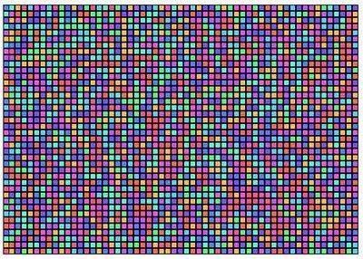
See a vertical stripe, what you are seeing is a run of repeated digits, like 7777, 00000, or 222.

One occurs in the top left:

Sequences like this used to be important examples in motivating discussions about the law of the excluded middle. Statements like: ‘the decimal expansion of pi contains the sequence 7777’, according to the law of the excluded middle, are either true or false. But when you are discussing something that has never been calculated, and that might never be calculated, suggests (to constructivists), that the statement may be neither true or false, and that the sequence 7777 may be somewhat like Schrodinger’s cat, neither existing nor not existing.

Now that the digits of pi have been calculated to astounding lengths, and that mathematics exists to uncover the properties of the pi digit sequence, the expansion of pi is no longer an ideal candidate for constructivist thought experiments. Even some exotic questions about the decimal expansion of pi, like the convergence of the brouwer-heyting sequence, have been resolved. Questions about the expansion of pi that illustrate constructivist problems can still be formulated, but they need to be more complicated than they used to be.

Still, I decided to look more closely at this little sequence that occurs (relatively) early on in the pi expansion. The stripe in the pi colour map mentioned above corresponds to the sequence 999999 beginning at digit 763 and ending at digit 768. This was observed in a set of the first 2281 digits of pi.

I decided to push the software a bit further, and load 10000 digits of pi into the document.  (A file with the first 10000 digits of pi formatted for Fathom or TinkerPlots is here.) The plot below shows the digits with 9 in black and all other digits blanked out – dots are single occurrences of a 9, while vertical stripes are runs of repeated 9s.

Using Tinkerplots’ runLength function we can see how frequent runs of various lengths are, and easily identify the longer ones.

Even with 10000 digits, the 999999 sequence at digit 763 was still the longest sequence of repeated digits. The other runner-up sequences in this first 10000 digits are, two instances of 2222, a single run of 8888, and four distinct occurrences of 7777.

The plot at the bottom of this post shows the distribution of even and odd digits in the decimal expansion of pi’s first 10000 digits, and was inspired by a similar plot from Wolfram Math World.

For more such insights, log into www.international-maths-challenge.com.

*Credit for article given to dan.mackinnon*


Monty Hall and the Three Prisoners

Brian Hayes recently provided some evidence that there are still many out there who are confounded by the Monty Hall problem.

The Monty Hall problem, perhaps the best-known counter-intuitive probability problem, gets a nice treatment in Jeffery Rosenthal’s Struck by Lightning: The Curious World of Probabilities, and is also explained well (perhaps better) in Mark Haddon’s novel The Curious Incident of the Dog in the Night-time. Professor Rosenthal has some further Monty Hall explanations here.

I just found an alternate version of the problem in Martin Gardner’s The Second Scientific American Book of Mathematical Puzzles and Diversions (published also by Penguin in a slightly different form as More Mathematical Puzzles and Diversions). In the chapter “Probability and Ambiguity” (chapter 19 in both versions of the book), Gardner describes the problem of the three prisoners. Here is a condensed description of the problem:

Three prisoners, A, B, and C are in separate cells and sentenced to death. The governor has selected one of them at random to be pardoned. Finding out that one is to be released, prisoner A begs the warden to let him know the identity of one of the others who is going to be executed. “If B is to be pardoned, give me C’s name. If C is to be pardoned, give me B’s name. And if I’m to be pardoned, flip a coin to decide whether to name B or C.”

The warden tells A that B is to be executed. Prisoner A is pleased because he believes that his probability of surviving has gone up from 1/3 to 1/2. Prisoner A secretly tells C the news, who is also happy to hear it, believing that his chance of survival has also risen to 1/2.

Are A and C correct? No. Prisoner A’s probability of surviving is still 1/3, but prisoner C’s probability of receiving the pardon is 2/3.

It is reasonably easy to see that the 3 prisoners problem is the same as the Monty Hall problem. Seeing the problem in this different formulation might help those who continue to struggle with it.

It is a nice activity to simulate both the 3 prisoners problem and the Monty Hall problem in Fathom – try it and confirm the surprising results that the “second prisoner” is pardoned 2/3 of the time, and that 2/3 of the time, the winning curtain is not the one you selected first.

There are many, many, ways to write these simulations. Here are the attributes and formulas for a Fathom implementation of the three prisoners:

The table below (click on it to see a larger version) shows a separate simulation for the Monty Hall problem. Here we are assuming three curtains “1”, “2”, and “3”, one of which has a prize behind it. You pick one, and then Monty reveals the contents behind one of the other curtains (the curtain with the prize behind it is not shown). In the game, you have the option of switching your choice for the curtain that has not been revealed.

After creating the attributes, you can “run the simulation” by adding data to the collection (Collection->New Cases…), the more the better.

Incidentally, Gardner’s use of A, B, and C reminds me of Stephen Leacock’s “A, B, and C: The Human Element in Mathematics.”

Addendum

A quick search shows that the connection between the Monty Hall problem and the Three Prisoners is well known (see the wikipedia entries on Monty Hall and the Three Prisoners), and that both are alternate formulations of an older problem, known as Bertrand’s box paradox.

For more such insights, log into www.international-maths-challenge.com.

*Credit for article given to dan.mackinnon*