Author: IMC

This post is the second example in an ongoing list of various sequences of functions which converge to different things in different ways.

‍Example 2

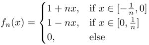
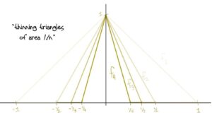
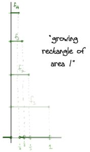
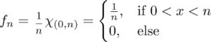
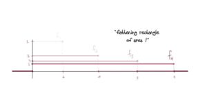
A sequence of functions {fn:R→R}{fn:R→R} which converges to 0 uniformly but does not converge to 0 in L1L1.

This works because:  The sequence tends to 0 as n→∞n→∞ since the height of each function tends to 0 and the the region where fnfn is taking on this decreasing height is tending towards all of R+R+ ((0,n)(0,n) as n→∞n→∞) (and it’s already 0 on R−∪{0}R−∪{0}). The convergence is uniform because the number of times we have to keep “squishing” the rectangles until their height is less than ϵϵ does not depend on xx.

The details: Let ϵ>0ϵ>0 and choose N∈NN∈N so that N>1ϵN>1ϵ and let n>Nn>N. Fix x∈Rx∈R.

Case 1 (x≤0x≤0 or x≥nx≥n) Then fn(x)=0fn(x)=0 and so |fn(x)−0|=0<ϵ|fn(x)−0|=0<ϵ.

• Case 2 (0<x<n0<x<n ) Then fn(x)=1nfn(x)=1n and so |fn(x)−0|=1n<1N<ϵ|fn(x)−0|=1n<1N<ϵ

Finally, fn↛0fn↛0 in L1L1 since∫R|fn|=∫(0,n)1n=1nλ((0,n))=1.∫R|fn|=∫(0,n)1n=1nλ((0,n))=1.

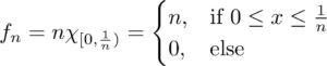
‍Remark: Here’s a question you could ask: wouldn’t fn=nχ(0,1n)fn=nχ(0,1n) work here too? Both are tending to 0 everywhere and both involve rectangles of area 1. The answer is “kinda.” The problem is that the convergence of nχ(0,1n)nχ(0,1n) is pointwise. BUT Egoroff’s Theorem gives us a way to actually “make” it uniform!.

‍On the notation above:   For a measurable set X⊂RX⊂R, denote the set of all Lebesgue integrable functions f:X→Rf:X→R by L1(X)L1(X). Then a sequence of functions {fn}{fn} is said to converge in L1L1  to a function ff if limn→∞∫|fn−f|=0limn→∞∫|fn−f|=0.

For more such insights, log into www.international-maths-challenge.com.

*Credit for article given to Tai-Danae Bradley*

Given a sequence of real-valued functions {fn}{fn}, the phrase, “fnfn converges to a function ff” can mean a few things:

• fnfn converges uniformly
• fnfn converges pointwise
• fnfn converges almost everywhere (a.e.)
• fnfn converges in L1L1 (set of Lebesgue integrable functions)
• and so on…

Other factors come into play if the fnfn are required to be continuous, defined on a compact set, integrable, etc.. So since I do not have the memory of an elephant (whatever that phrase means…), I’ve decided to keep a list of different sequences that converge (or don’t converge) to different functions in different ways. With each example I’ll also include a little (and hopefully) intuitive explanation for why. Having these sequences close at hand is  especially useful when analysing the behavior of certain functions or constructing counterexamples.

The first sequence we’ll look at is one which converges almost everywhere, but does not converge in L1L1 (the set of Lebesgue integrable functions).

‍Example 1

A sequence of functions {fn:R→R}{fn:R→R} which converges to 0 almost everywhere but does not converge to 0 in L1L1.       

This works because: Recall that to say fn→0fn→0 almost everywhere means fn→0fn→0 pointwise on RR except for a set of measure 0. Here, the set of measure zero is the singleton set {0}{0} (at x=0x=0, fn(x)=nfn(x)=n and we can’t make this less than ϵϵ for any ϵ>0ϵ>0). So fnfn converges to 0 pointwise on (0,1](0,1]. This holds because if x<0x<0 or x>1x>1 then fn(x)=0fn(x)=0 for all nn. Otherwise, if x∈(0,1]x∈(0,1], we can choose nn appropriately:

The details:  Let ϵ>0ϵ>0 and x∈(0,1]x∈(0,1] and choose N∈NN∈N so that N>1xN>1x. Then whenever n>Nn>N, we have n>1xn>1x which implies x>1nx>1n and so fn(x)=0fn(x)=0. Hence |fnx−0|=0<ϵ|fnx−0|=0<ϵ.

Further*, fn↛0fn↛0 in L1L1 since∫R|fn|=∫[0,1n]n=nλ([0,1n])=1.∫R|fn|=∫[0,1n]n=nλ([0,1n])=1.

Remark: Notice that Egoroff’s theorem applies here! We just proved that fn→0fn→0 pointwise a.e. on RR, but Egoroff says that we can actually get uniform convergence a.e. on a bounded subset of RR, say (0,1](0,1].

In particular for each ϵ>0ϵ>0 we are guaranteed the existence of a subset E⊂(0,1]E⊂(0,1] such that fn→0fn→0 uniformly and λ((0,1]∖E)<ϵλ((0,1]∖E)<ϵ. In fact, it should be clear that that subset must be something like (ϵ2,1](ϵ2,1] (the “zero region” in the graph above). Then no matter where xx is in (0,1](0,1], we can always find nn large enough – namely all nn which satisfy 1n<ϵ21n<ϵ2 – so that fn(x)=0fn(x)=0, i.e. fn→ffn→f uniformly. And indeed, λ((0,1]∖(ϵ2,1]=ϵ/2<ϵλ((0,1]∖(ϵ2,1]=ϵ/2<ϵ as claimed.

‍On the notation above:   For a measurable set X⊂RX⊂R, denote the set of all Lebesgue integrable functions f:X→Rf:X→R by L1(X)L1(X). Then a sequence of functions {fn}{fn} is said to converge in L1L1  to a function ff if limn→∞∫|fn−f|=0limn→∞∫|fn−f|=0.

For more such insights, log into www.international-maths-challenge.com.

*Credit for article given to Tai-Danae Bradley*

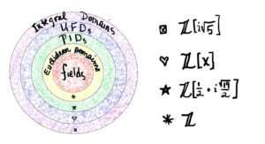
In any area of math, it’s always good idea to keep a few counterexamples in your back pocket. Examples/non-examples from some of the different subsets of integral domains.

Z[i√5]Z[i5] is an integral domain which is not a UFD

That Z[i√5]Z[i5] an integral domain is easy to check (just computation).

• It’s not a UFD since we can write 6=2⋅3=(1+i√5)(1−i√5)6=2⋅3=(1+i5)(1−i5) as two distinct facorizations into irreducibles*

‍Z[x]Z[x] is a UFD which is not a PID

We know Z[x]Z[x] is a UFD because ZZ is a UFD (recall, a commutative ring RR is a UFD iff R[x]R[x] is a UFD).

• The ideal (2,x)={2f(x)+xg(x):f(x),g(x)∈Z[x]}(2,x)={2f(x)+xg(x):f(x),g(x)∈Z[x]} (polynomials with even constant term) is not principal**

‍Z[12+i√192]Z[12+i192] is a PID which is not a Euclidean domain

• This is a PID since it has a Dedekind-Hasse norm (see Dummit and Foote, 3rd ed., §8.2§8.2).
• It is not a Euclidean domain since it has no universal side divisors (ibid.).

ZZ is a Euclidean domain which is not a field

ZZ is a Euclidean domain via the absolute value norm (which gives the familiar division algorithm).

• It is not a field since the only elements which are units are 11 and −1−1.

‍  (*) Check 2,3,1+i√52,3,1+i5, and 1−i√51−i5 are indeed irreducible in Z[i√5]Z[i5]:

Write 2=αβ2=αβ for α,β∈Z[i√5]α,β∈Z[i5]. Then α=a+ib√5α=a+ib5 and N(α)=a2+5b2N(α)=a2+5b2 for some integers a,ba,b. Since 4=N(2)=N(α)N(β)4=N(2)=N(α)N(β), we must have a2+5b2=1,2a2+5b2=1,2 or 44. Notice b=0b=0 must be true (since a2+5b2∉{1,2,4}a2+5b2∉{1,2,4} for b≥1b≥1 and for any aa). Hence either α=a=1α=a=1 or 22. If α=1α=1 then αα is a unit. If α=2α=2, then we must have β=1β=1 and so ββ is a unit.

• Showing 3 is irreducible follows a similar argument.

‍Write 1+i√5=αβ1+i5=αβ with α=a+ib√5α=a+ib5 so that N(α)=a2+5b2∈{1,2,3,6}N(α)=a2+5b2∈{1,2,3,6} since 6=N(α)N(β)6=N(α)N(β). Consider two cases:  (case 1) If b=0b=0, then a2∈{1,2,3,6}a2∈{1,2,3,6} which is only true if a2=1a2=1 and so α=a=±1α=a=±1 is a unit. (case 2) If b>0b>0, we can only have b2=1b2=1 (since b2>1b2>1 gives a contradiction), and so a2+5∈{1,2,3,6}a2+5∈{1,2,3,6}, which implies a2=1a2=1. Hence α=±1±i√5α=±1±i5 and so N(α)=6N(α)=6. This implies N(β)=1N(β)=1 and so β=±1β=±1, which is a unit.

‍Showing 1−i√51−i5 is irreducible follows a similar argument.

principal in Z[x]Z[x]:

• Suppose to the contrary (2,x)=(f(x))(2,x)=(f(x)) for some polynomial f(x)∈Z[x]f(x)∈Z[x]. Since 2∈(f(x))2∈(f(x)), we must have 2=f(x)p(x)2=f(x)p(x) for some p(x)∈Z[x]p(x)∈Z[x]. Hence 0=degf(x)+degp(x)0=deg⁡f(x)+deg⁡p(x) which implies both f(x)f(x) and p(x)p(x) are constants. In particular, since 2=±1⋅±22=±1⋅±2, we need f(x),p(x)∈{±1,±2}f(x),p(x)∈{±1,±2}. If f(x)=±1f(x)=±1, then (f(x))=Z[x](f(x))=Z[x] which is a contradiction since (f(x))=(2,x)(f(x))=(2,x) mustbe a proper ideal (not every polynomial over Z[x]Z[x] has even constant term). It follows that f(x)=±2f(x)=±2. But since x∈(f(x))x∈(f(x)) as well, x=2r(x)x=2r(x) for some r(x)∈Z[x]r(x)∈Z[x]. But of course this is impossible for any polynomial with integer coefficients, r(x)r(x). Thus (2,x)(2,x) is not principal.

For more such insights, log into www.international-maths-challenge.com.

*Credit for article given to Tai-Danae Bradley*

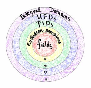
Here is a list of some of the subsets of integral domains, along with the reasoning (a.k.a proofs) of why the bullseye below looks the way it does. Part 2 of this post will include back-pocket examples/non-examples of each.

Integral Domain: a commutative ring with 1 where the product of any two nonzero elements is always nonzero

Unique Factorization Domain (UFD): an integral domain where every nonzero element (which is not a unit) has a unique factorization into irreducibles

Principal Ideal Domain (PID): an integral domain where every ideal is generated by exactly one element

Euclidean Domain: an integral domain RR with a norm NN and a division algorithm (i.e. there is a norm NN so that for every a,b∈Ra,b∈R with b≠0b≠0, there are q,r∈Rq,r∈R so that a=bq+ra=bq+r with r=0r=0 or N(r)<N(b)N(r)<N(b))

Field: a commutative ring where every nonzero element has an inverse

Because… We can just choose the zero norm: N(r)=0N(r)=0 for all r∈Fr∈F.

Proof: Let FF be a field and define a norm NN so that N(r)=0N(r)=0 for all r∈Fr∈F. Then for any a,b∈Fa,b∈F with b≠0b≠0, we can writea=b(b−1a)+0.a=b(b−1a)+0.

Because… If I◃RI◃R is an arbitrary nonzero ideal in the Euclidean domain RR, then I=(d)I=(d), where d∈Id∈I such that dd has the smallest norm among all elements in II. Prove this using the division algorithm on dd and some a∈Ia∈I.

Proof: Let RR be a Euclidean domain with respect to the norm NN and let I◃RI◃R be an ideal. If I=(0)I=(0), then II is principle. Otherwise let d∈Id∈I be a nonzero element such that dd has the smallest norm among all elements in II. We claim I=(d)I=(d). That (d)⊂I(d)⊂I is clear so let a∈Ia∈I. Then by the division algorithm, there exist q,r∈Rq,r∈R so that a=dq+ra=dq+r with r=0r=0 or N(r)<N(d)N(r)<N(d). Then r=a−dq∈Ir=a−dq∈I since a,d∈Ia,d∈I. But my minimality of dd, this implies r=0r=0. Hence a=dq∈(d)a=dq∈(d) and so I⊂(d)I⊂(d).

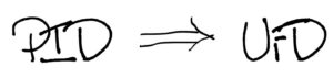
Because…Every PID has the ascending chain condition (acc) on its ideals!* So to prove PID ⇒⇒ UFD, just recall that an integral domain RR is a UFD if and only if 1) it has the acc on principal ideals** and 2) every irreducible element is also prime.

Proof: Let RR be a PID. Then 1) RR has the ascending chain condition on principal ideals and 2) every irreducible element is also a prime element. Hence RR is a UFD.

Because… By definition.

Proof: By definition.

‍*Def: In general, an integral domain RR has the acc on its principal ideals if these two equivalent conditions are satisfied:

1. Every sequence I1⊂I2⊂⋯⊂⋯I1⊂I2⊂⋯⊂⋯ of principal ideals is stationary (i.e. there is an integer n0≥1n0≥1 such that In=In0In=In0 for all n≥n0n≥n0).
2. For every nonempty subset X⊂RX⊂R, there is an element m∈Xm∈X such that whenever a∈Xa∈X and (m)⊂(a)(m)⊂(a), then (m)=(a)(m)=(a).

**To see this, use part 1 of the definition above. If I1⊂I2⊂⋯I1⊂I2⊂⋯ is an acsending chain, consider their union I=⋃∞n=1InI=⋃n=1∞In. That guy must be a principal ideal (check!), say I=(m)I=(m). This implies that mm must live in some In0In0  for some n0≥1n0≥1 and so I=(m)⊂In0I=(m)⊂In0. But since II is the union, we have for all n≥n0n≥n0(m)=I⊃In⊃In0=(m).(m)=I⊃In⊃In0=(m).Voila!

Every field FF is a PID

because the only ideals in a field are (0)(0) and F=(1)F=(1)! And every field is vacuously a UFD since all elements are units. (Recall, RR is a UFD if every non-zero, non-invertible element (an element which is not a unit) has a unique factorzation into irreducibles).

‍In an integral domain, every maximal ideal is also a prime ideal. 

(Proof: Let RR be an integral domain and M◃RM◃R a maximal ideal. Then R/MR/M is a field and hence an integral domain, which implies M◃RM◃R is a prime ideal.)

Butut the converse is not true (see counterexample below). However, the converse is true in a PID because of the added structure!

(Proof: Let RR be a PID and (p)◃R(p)◃R a prime ideal for some p∈Rp∈R. Then pp is a prime – and hence an irreducible – element (prime ⇔⇔ irreducible in PIDs). Since in an integral domain a principal ideal is maximal whenever it is generated by an irreducible element, we conclude (p)(p) is maximal.)

This suggests that if you want to find a counterexample – an integral domain with a prime ideal which is not maximal – try to think of a ring which is not a PID:   In Z[x]Z[x], consider the ideal (p)(p) for a prime integer pp. Then (p)(p) is a prime ideal, yet it is not maximal since(p)⊂(p,x)⊂Z[x].(p)⊂(p,x)⊂Z[x].

‍If FF is a field, then F[x]F[x] – the ring of polynomials in xx with coefficients in FF – is a Euclidean domain with the norm N(p(x))=degp(x)N(p(x))=deg⁡p(x) where p(x)∈F[x]p(x)∈F[x].

By the integral domain hierarchy above, this implies every ideal in F[x]F[x] is of the form (p(x))(p(x)) (i.e. F[x]F[x] is a PID) and every polynomial can be factored uniquely into a product of prime polynomials (just like the integers)! The next bullet gives an “almost converse” statement.

‍If R[x]R[x] is a PID, the RR must be a field.

To see this, simply observe that R⊂R[x]R⊂R[x] and so RR must be an integral domain (since a subset of a integral domain inherets commutativity and the “no zero divisors” property). Since R[x]/(x)≅RR[x]/(x)≅R, it follows that R[x]/(x)R[x]/(x) is also an integral domain. This proves that (x)(x) is a prime ideal. But prime implies maximal in a PID! So R[x]/(x)R[x]/(x) – and therefore RR – is actually a field.

• This is how we know, for example, that Z[x]Z[x] is not a PID (in the counterexample a few bullets up) – ZZ is not a field!

‍For more such insights, log into www.international-maths-challenge.com.

*Credit for article given to Tai-Danae Bradley*

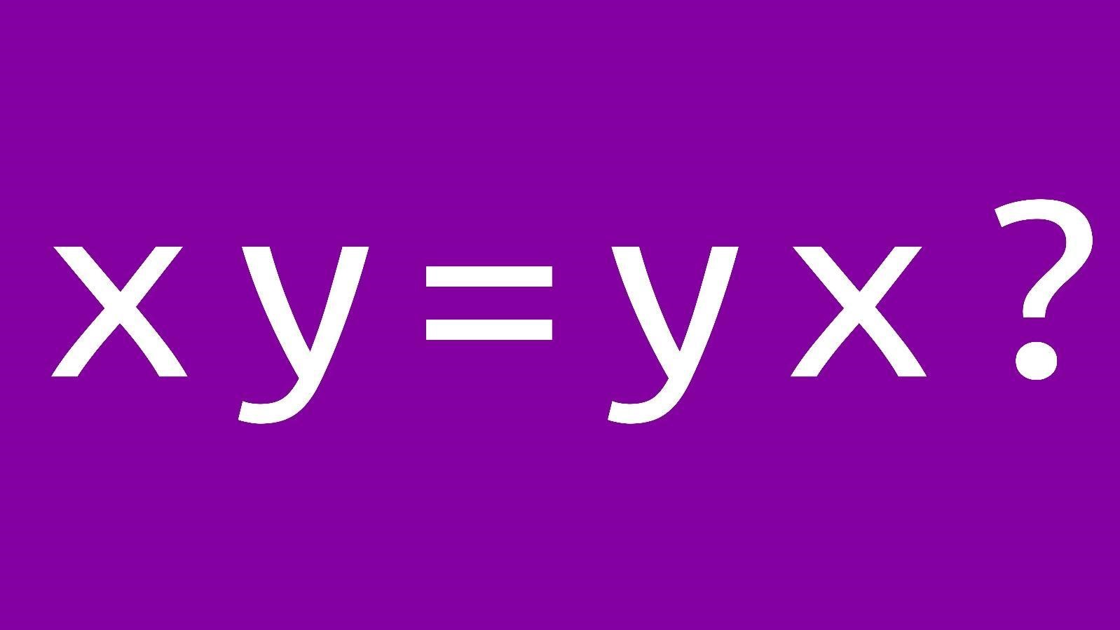
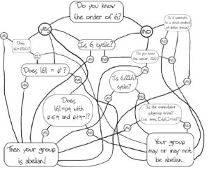
After some exposure to group theory, you quickly learn that when trying to prove a group GG is abelian, checking if xy=yxxy=yx for arbitrary x,yx,y in GG is not always the most efficient – or helpful! – tactic. Here is a (not comprehensive) running tab of other ways you may be able to prove your group is abelian:

Show the commutator [x,y]=xyx−1y−1[x,y]=xyx−1y−1of two arbitary elements x,y∈Gx,y∈G must be the identity

• Show the group is isomorphic to a direct product of two abelian (sub)groups
• Check if the group has order p2p2 for any prime pp OR if the order is pqpq for primes p≤qp≤q with p∤q−1p∤q−1.
• Show the group is cyclic.
• Show |Z(G)|=|G|.|Z(G)|=|G|.
• Prove G/Z(G)G/Z(G) is cyclic. (e.g. does G/Z(G)G/Z(G) have prime order?)
• Show that GG has a trivial commutator subgroup, i.e. is [G,G]={e}[G,G]={e}.

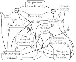
Here’s a thought map which is (probably) more fun than practical. Note, pp and qq denote primes below:

For more such insights, log into www.international-maths-challenge.com.

*Credit for article given to Tai-Danae Bradley*

Yes! I’m writing about math. No! Don’t close your browser window. Hear me out first…

I know very well that math has a bad rap. It’s often taught or thought of as a dry, intimidating, unapproachable, completely boring, who-in-their-right-mind-would-want-to-think-about-this-on-purpose kind of subject. I get it. Math was the last thing on earth I thought I’d study. Seriously.

But my understanding of math has since changed. I used to think it was a mess of equations and formulas, only enjoyed by a small number of masochists. But oh how I was wrong! Mathematics is not just numbers. It is not just strange symbols. And it is certainly not something reserved only for the few elite geniuses of the world.

Mathematics is a language –

a language of ideas, concepts, and notions.

‍

It’s true! Math is a language just like English, French, or Mandarin. And just like some ideas are best communicated in a particular language, other ideas are best communicated “in math.” This is why I’ve started a SaiBlog – as an aid in my own pursuit of becoming more proficient at thinking/speaking/reading mathematics.

One of the main challenges I face in this pursuit is the ability to strip away the intimidation factor

– the cryptic symbols, the elaborate vocabulary, the fancy formalities –

and unveil the true meaning of the text at hand. For me, this unveiling comes by reading and rereading, by working through problem after problem, and by writing. Quite often while learning new (and recalling old) mathematics, I have to stop and ask, “What is the text really saying behind all that jargon?” And if I can proceed to write down the idea in English (i.e. in lingo that’s easy on the brain) then that bit of information becomes engrained in my mind. Or at least it gets stored away in my brain somewhere. And if (or when) I forget it, I find that looking at my own handwritten notes conjures up the memory and the blood, sweat, and tears that went into learning that bit of info, and it all comes right back.

So Math3ma is my online repository as I make my way through this journey. Here’s the plan for now: some of the SaiBlog posts will be divided into two sections, in keeping with the aforementioned thought process:

And some posts will fall into “The Back Pocket” where I’ll keep little tidbits of math for a rainy day (or, perhaps, an exam). As for the actual content, I’m focusing on material found in the initial years of a graduate math program because, well, passing the qualifying exams is next on my agenda. But I think I’ll include some include undergrad material too. And as for future content, who knows? I’m excited to see what Math3ma can turn into.

Thanks for taking the time to peak into my journey as I work to see mathematics for what it really is–a very powerful, very beautiful language inherent in the world all around us!

For more such insights, log into www.international-maths-challenge.com.

*Credit for article given to Tai-Danae Bradley*

Bob Moses, who helped register Black residents to vote in Mississippi during the Civil Rights Movement, believed civil rights went beyond the ballot box. To Moses, who was a teacher as well as an activist, math literacy is a civil right: a requirement to earning a living wage in modern society. In 1982, he founded the Algebra Project to ensure that “students at the bottom get the math literacy they need.”

As a researcher who studies ways to improve the math experiences of students, we believe a new approach that expands access to algebra may help more students get the math literacy Moses, who died in 2021, viewed as so important. It’s a goal districts have long been struggling to meet.

Efforts to improve student achievement in algebra have been taking place for decades. Unfortunately, the math pipeline in the United States is fraught with persistent opportunity gaps. According to the Nation’s Report Card—a congressionally mandated project administered by the Department of Education—in 2022 only 29% of U.S. fourth graders and 20% of U.S. eighth graders were proficient in math. Low-income students, students of colour and multilingual learners, who tend to have lower scores on math assessments, often do not have the same access as others to qualified teachers, high-quality curriculum and well-resourced classrooms.

A new approach

The Dallas Independent School District—or Dallas ISD—is gaining national attention for increasing opportunities to learn by raising expectations for all students. Following in the footsteps of more than 60 districts in the state of Washington, in 2019 the Dallas ISD implemented an innovative approach of having students be automatically enrolled rather than opt in to honours math in middle school.

Under an opt-in policy, students need a parent or teacher recommendation to take honours math in middle school and Algebra 1 in eighth grade. That policy led both to low enrolment and very little diversity in honours math. Some parents, especially those who are Black or Latino, were not aware how to enroll their students in advanced classes due to a lack of communication in many districts.

In addition, implicit bias, which exists in all demographic groups, may influence teachers’ perceptions of the behaviour and academic potential of students, and therefore their subsequent recommendations. Public school teachers in the U.S. are far less racially and ethnically diverse than the students they serve.

Dallas ISD’s policy overhaul aimed to foster inclusivity and bridge educational gaps among students. Through this initiative, every middle school student, regardless of background, was enrolled in honours math, the pathway that leads to taking Algebra 1 in eighth grade, unless they opted out.

Flipping the switch from opt-in to opt-out led to a dramatic increase in the number of Black and Latino learners, who constitute the majority of Dallas students. And the district’s overall math scores remained steady. About 60% of Dallas ISD eighth graders are now taking Algebra 1, triple the prior level. Moreover, more than 90% are passing the state exam.

Efforts spread

Other cities are taking notice of the effects of Dallas ISD’s shifting policy. The San Francisco Unified School District, for example, announced plans in February 2024 to implement Algebra 1 in eighth grade in all schools by the 2026-27 school year.

In fall 2024, the district will pilot three programs to offer Algebra 1 in eighth grade. The pilots range from an opt-out program for all eighth graders—with extra support for students who are not proficient—to a program that automatically enrolls proficient students in Algebra 1, offered as an extra math class during the school day. Students who are not proficient can choose to opt in. Nationwide, however, districts that enroll all students in Algebra 1 and allow them to opt out are still in the minority. And some stopped offering eighth grade Algebra 1 entirely, leaving students with only pre-algebra classes. Cambridge, Massachusetts—the city in which Bob Moses founded the Algebra Project—is among them.

Equity concerns linger

Between 2017 and 2019, district leaders in the Cambridge Public Schools phased out the practice of placing middle school students into “accelerated” or “grade-level” math classes. Few middle schools in the district now offer Algebra 1 in eighth grade.

The policy shift, designed to improve overall educational outcomes, was driven by concerns over significant racial disparities in advanced math enrollment in high school. Completion of Algebra 1 in eighth grade allows students to climb the math ladder to more difficult classes, like calculus, in high school. In Cambridge, the students who took eighth grade Algebra 1 were primarily white and Asian; Black and Latino students enrolled, for the most part, in grade-level math.

Some families and educators contend that the district’s decision made access to advanced math classes even more inequitable. Now, advanced math in high school is more likely to be restricted to students whose parents can afford to help them prepare with private lessons, after-school programs or private schooling, they said.

While the district has tried to improve access to advanced math in high school by offering a free online summer program for incoming ninth graders, achievement gaps have remained persistently wide.

Perhaps striking a balance between top-down policy and bottom-up support will help schools across the U.S. realize the vision Moses dreamed of in 1982 when he founded the Algebra Project: “That in the 21st century every child has a civil right to secure math literacy—the ability to read, write and reason with the symbol systems of mathematics.”

For more insights like this, visit our website at www.international-maths-challenge.com.

Credit of the article given to Liza Bondurant, The Conversation

The colorful leaves piling up in your backyard this fall can be thought of as natural stores of carbon. In the springtime, leaves soak up carbon dioxide from the atmosphere, converting the gas into organic carbon compounds. Come autumn, trees shed their leaves, leaving them to decompose in the soil as they are eaten by microbes. Over time, decaying leaves release carbon back into the atmosphere as carbon dioxide.

In fact, the natural decay of organic carbon contributes more than 90 percent of the yearly carbon dioxide released into Earth’s atmosphere and oceans. Understanding the rate at which leaves decay can help scientists predict this global flux of carbon dioxide, and develop better models for climate change. But this is a thorny problem: A single leaf may undergo different rates of decay depending on a number of variables: local climate, soil, microbes and a leaf’s composition. Differentiating the decay rates among various species, let alone forests, is a monumental task.

Instead, MIT researchers have analysed data from a variety of forests and ecosystems across North America, and discovered general trends in decay rates among all leaves. The scientists devised a mathematical procedure to transform observations of decay into distributions of rates. They found that the shape of the resulting curve is independent of climate, location and leaf composition. However, the details of that shape—the range of rates that it spans, and the mean rate—vary with climatic conditions and plant composition. In general, the scientists found that plant composition determines the range of rates, and that as temperatures increase, all plant matter decays faster.

“There is a debate in the literature: If the climate warms, do all rates become faster by the same factor, or will some become much faster while some are not affected?” says Daniel Rothman, a co-founder of MIT’s Lorenz Center, and professor of geophysics in the Department of Earth, Atmospheric and Planetary Sciences. “The conclusion is that all rates scale uniformly as the temperature increases.”

Rothman and co-author David Forney, a PhD graduate in the Department of Mechanical Engineering, have published the results of their study, based largely on Forney’s PhD thesis, in the Journal of the Royal Society Interface.

Litter delivery

The team obtained data from an independent 10-year analysis of North American forests called the Long-term Intersite Decomposition Experiment Team (LIDET) study. For this study, researchers collected leaf litter—including grass, roots, leaves and needles—from 27 locations throughout North and Central America, ranging from Alaskan tundra to Panamanian rainforests.

The LIDET researchers separated and weighed each litter type, and identified litter composition and nutrient content. They then stored the samples in porous bags and buried the bags, each filled with a different litter type, in each of the 27 geographic locations; the samples were then dug up annually and reweighed. The data collected represented the mass of litter, of different composition, remaining over time in different environments.

Forney and Rothman accessed the LIDET study’s publicly available data online, and analysed each dataset: the litter originating at one location, subsequently divided and distributed at 27 different locations, and weighed over 10 years.

The team developed a mathematical model to convert each dataset’s hundreds of mass measurements into rates of decay—a “numerically delicate” task, Rothman says. They then plotted the converted data points on a graph, yielding a surprising result: The distribution of decay rates for each dataset looked roughly the same, forming a bell curve when plotted as a function of the order of magnitude of the rates—a surprisingly tidy pattern, given the complexity of parameters affecting decay rates.

“Not only are there different environments like grasslands and tundra and rainforest, there are different environments at the microscale too,” Forney says. “Each plant is made up of different tissues … and these all have different degradation pathways. So there’s heterogeneity at many different scales … and we’re trying to figure out if there’s some sort of commonality.”

Common curves

Going a step further, Forney and Rothman looked for parameters that affect leaf decay rates. While each dataset resembled a bell curve, there were slight variations among them. For example, some curves had higher peaks, while others were flatter; some curves shifted to the left of a graph, while others lay more to the right. The team looked for explanations for these slight variations and discovered the two parameters that most affected the details of a dataset’s curve: climate and leaf composition.

In general, the researchers observed, warmer climates tended to speed the decay of all plants, whereas colder climates slowed plant decay uniformly. The implication is that as temperatures increase, all plant matter, regardless of composition, will decay more quickly, with the same relative speedup in rate.

The team also found that plant matter such as needles that contain more lignin—a sturdy building block—have a smaller range or decay rates than leafier plants that contain less lignin and more nutrients that attract microbes. “This is an interesting ecological finding,” Forney says. “Lignin tends to shield organic compounds, which may otherwise degrade at a faster rate.”

Mark Harmon, principal investigator for the LIDET study and a professor of forest science at Oregon State University, says the team’s results add evidence to a long-held debate over rising temperature’s effect on organic decay: As temperatures rise, decomposition will likely speed up, releasing more carbon dioxide into the atmosphere, which in turn creates warmer temperatures, further speeding decay in a positive feedback loop.

“There is a wide range of results on temperature response,” says Harmon, who was not involved in the study. “Some have proposed that materials that are hard to decompose will respond more to temperature increases, and others have proposed the opposite. The current study indicates they may be the same,” meaning the positive feedback from rising temperatures may not be as strong as others have predicted.

Rothman adds that in the future, the team may use the model to predict the turnover times of various ecosystems — a finding that may improve climate change models, and help scientists understand the flux of carbon dioxide around the globe.

Rothman adds that in the future, the team may use the model to predict the turnover times of various ecosystems—a finding that may improve climate change models, and help scientists understand the flux of carbon dioxide around the globe.

“It’s a really messy problem,” Rothman says. “It’s as messy as the pile of leaves in your backyard. You would think that each pile of leaves is different, depending on which tree it’s from, where the pile is in your backyard and what the climate is like. What we’re showing is that there’s a mathematical sense in which all of these piles of leaves behave in the same way.”

For more such insights, log into our website https://international-maths-challenge.com

Credit of the article given to Jennifer Chu, Massachusetts Institute of Technology

People love to complain about the weather – and especially about weather forecasters. But real, accurate forecasting beyond five to seven days is immensely complicated, due to the sheer volume of atmospheric processes and factors. Fortunately for us, advances in computing are making it possible for mathematicians, atmospheric scientists and statisticians to create “models of everything,” which may lead to accurate long-range weather forecasts.

NC State mathematician John Harlim is working on one such “model of everything,” specifically for longer-range weather and climate prediction. He’s part of a five-year project led by NYU’s Andrew Majda that is creating simpler, less expensive stochastic models (a model that includes random variables) for extended range weather and climate prediction.

One major stumbling block to extending and improving weather predictions beyond seven-day forecasts is a lack of understanding of the tropical weather dynamics that drive global weather patterns. The mix of factors in these patterns is amazingly complex. According to Harlim, “The dynamics in the tropics involve hierarchies of processes on both huge scales – like, 10,000 km – and much smaller scales over many months.  Physical processes in individual clouds can affect these larger processes in the long run.

“In terms of a model, then, you would have to resolve the entire globe in one-kilometer chunks, look at every possible weather pattern that could possibly occur over every moment given all sorts of variables, and then scale it up,” Harlim adds. Since this approach is very expensive, computationally speaking, Harlim and his colleagues hope to develop simpler, cheaper models that can capture tropical dynamics and understand their interactions with extratropical weather patterns.

Says Harlim, “Understanding tropical dynamics is the Holy Grail of atmospheric modeling, and if we’re successful, you’ll be able to get accurate weather forecasting for months, not just days, in advance.”

Atmospheric scientist Sukanta Basu is part of a team working on a “model of everything” for atmospheric turbulence by studying airflow over complex terrain, including islands. The team wants to understand how atmospheric turbulence affects laser propagations, but their work could have other applications as well – such as predicting microbursts for aircraft safety or estimating evaporation rates for water management in agriculture. And just like Harlim’s, Basu’s model will have to take a huge number of factors into account.

“We’ll be looking at 10-meter terrain maps, finding out every spatial location and time and what the atmospheric field may look like,” Basu says. “The amount of computational power needed is huge – one simulation can fill up a terabyte disk – so we’re looking at petascale computing, which can do a quadrillion operations per second. We didn’t have computing on this scale ten years ago, so projects like this were impossible.”

For more such insights, log into our website https://international-maths-challenge.com

Credit of the article given to Tracey Peake, North Carolina State University

A team of EPFL scientists has developed an algorithm that can identify the source of an epidemic or information circulating within a network, a method that could also be used to help with criminal investigations.

Investigators are well aware of how difficult it is to trace an unlawful act to its source. The job was arguably easier with old, Mafia-style criminal organizations, as their hierarchical structures more or less resembled predictable family trees.

In the Internet age, however, the networks used by organized criminals have changed. Innumerable nodes and connections escalate the complexity of these networks, making it ever more difficult to root out the guilty party. EPFL researcher Pedro Pinto of the Audiovisual Communications Laboratory and his colleagues have developed an algorithm that could become a valuable ally for investigators, criminal or otherwise, as long as a network is involved.

“Using our method, we can find the source of all kinds of things circulating in a network just by ‘listening’ to a limited number of members of that network,” explains Pinto. Suppose you come across a rumor about yourself that has spread on Facebook and been sent to 500 people; your friends, or even friends of your friends. How do you find the person who started the rumor? “By looking at the messages received by just 15󈞀 of your friends, and taking into account the time factor, our algorithm can trace the path of that information back and find the source,” Pinto adds. This method can also be used to identify the origin of a spam message or a computer virus using only a limited number of sensors within the network.

Out in the real world, the algorithm can be employed to find the primary source of an infectious disease, such as cholera. “We tested our method with data on an epidemic in South Africa provided by EPFL professor Andrea Rinaldo’s Ecohydrology Laboratory,” says Pinto. “By modeling water networks, river networks, and human transport networks, we were able to find the spot where the first cases of infection appeared by monitoring only a small fraction of the villages.”

The method would also be useful in responding to terrorist attacks, such as the 1995 sarin gas attack in the Tokyo subway, in which poisonous gas released in the city’s subterranean tunnels killed 13 people and injured nearly 1,000 more. “Using this algorithm, it wouldn’t be necessary to equip every station with detectors. A sample would be sufficient to rapidly identify the origin of the attack, and action could be taken before it spreads too far,” says Pinto.

Computer simulations of the telephone conversations that could have occurred during the terrorist attacks on September 11, 2001, were used to test Pinto’s system. “By reconstructing the message exchange inside the 9/11 terrorist network extracted from publicly released news, our system spit out the names of three potential suspects; one of whom was found to be the mastermind of the attacks, according to the official enquiry.”

The validity of this method thus has been proven a posteriori. But according to Pinto, it could also be used preventatively; for example, to understand an outbreak before it gets out of control. “By carefully selecting points in the network to test, we could more rapidly detect the spread of an epidemic,” he points out. It could also be a valuable tool for advertisers who use viral marketing strategies by leveraging the Internet and social networks to reach customers. For example, this algorithm would allow them to identify the specific Internet that are the most influential for their target audience and to understand how in these articles spread throughout the online community.

For more such insights, log into our website https://international-maths-challenge.com

Credit of the article given to Ecole Polytechnique Federale de Lausanne