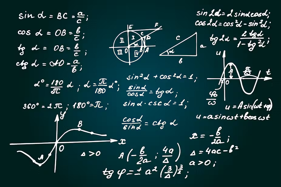
“The Danger of a Single Story” in Mathematics

Credit: George Coppock Getty Images

The Lathisms podcast shares the varied stories of Hispanic and Latinx mathematicians

Writer Chimamanda Ngozi Adichie’s popular TED talk is called “The danger of a single story.” In it, she talks about the importance of reading and writing many stories of many people rather than putting a person—or an entire continent of people—into one box. “The single story creates stereotypes,” she says, “and the problem with stereotypes is not that they are untrue but that they are incomplete.”

If someone were asked to tell the story of a “typical” mathematician, they might talk about a shy, socially awkward white man who is a “genius,” whatever that means. He was a fast learner in school and can perform feats of calculation almost instantaneously in his head. He thinks about nothing other than his research, often to the detriment of practical tasks required for everyday living. Some mathematicians do fit these descriptions, but many more don’t. When that story becomes the dominant narrative of who mathematicians are, people who don’t fit the mold feel like there’s no place for them in mathematics. One of the great privileges of working as a math writer is getting to hear the stories of so many mathematicians when I talk to them for articles or podcasts. There really is no one kind of person who becomes a mathematician.

This fall, I’m happy to share a project, created by Lathisms and sponsored by a Tensor-SUMMA grant from the Mathematical Association of America, to share more stories of mathematicians. Lathisms was founded in 2016 by four Hispanic mathematicians, Alexander Diaz-Lopez, Pamela Harris, Alicia Prieto Langarica, and Gabriel Sosa. Hispanic and Latinx people are underrepresented in mathematics, and Lathisms aims to increase visibility of Hispanic and Latinx mathematicians. Since 2016, the organizers have created a calendar every Hispanic Heritage month (September 15-October 15) where each day has a different featured Hispanic or Latinx mathematician, including a picture and short biography of each of them.

This year, Lathisms decided to extend the celebration of Hispanic and Latinx mathematicians by adding a podcast, hosted by me, where you can listen to these mathematicians tell their stories in their own words. Starting at the end of August, we have published a new episode every Friday. The episodes feature mathematicians featured in past years’ Lathisms calendars as well as some of this year’s mathematicians. Some of them grew up in the U.S., others in Latin America. Some grew up in poverty, and others were better off. Some knew they wanted to be mathematicians from a young age, and others didn’t know anything about possible mathematics careers until college. Some work in pure math, others in applied. Some focus on research, others outreach.

So far we’ve shared conversations with Carlos Castillo-Chavez, who is one of the most prolific advisors of U.S. Latinx math Ph.D. students; Erika Camacho, who does mathematical modeling of eye diseases; Federico Ardila, who mentioned “the danger of a single story” when we talked and finds inspiration and mentorship from both students and teachers; and Nicolas Garcia Trillos, who just started a new job in the statistics department at the University of Wisconsin Madison and talked about the many ways there are to be a good mathematician and how that helps him get “unstuck” in his works. In the coming weeks, we will share many more stories. Tune in on Fridays to find them.

You can find the podcast at the Lathisms website or on iTunes. Transcripts are available already for some episodes and will be provided for all episodes. I hope these conversations will be helpful for teachers who want to make sure their students are aware of the diversity of mathematicians, for Hispanic and Latinx students and early-career mathematicians who are looking for role models and collaborators, and for anyone who wants to hear about mathematicians’ many different stories.

For more insights like this, visit our website at www.international-maths-challenge.com.

Credit of the article given to Evelyn Lamb


The genius at Guinness and his statistical legacy

This St Patrick’s Day, revellers around the world will crowd the streets seeking one of Ireland’s national drinks: a pint of Guinness. But besides this tasty stout, one of the most fundamental and commonly used tools of science also has its origins at the Guinness brewery.

Towards the end of the 19th century, Guinness was scaling up its operations, and was interested in applying a scientific approach to all aspects of Guinness production: from barley growth right through to the Guinness taste.

Before adopting a scientific approach, brewers at Guinness relied on subjective methods, such as the appearance and scent of hops, to assess produce quality.

Once scientific brewers were recruited, a more objective approach was taken. The first scientific brewer, Thomas Bennett Case, was hired in 1893 and he believed that the amount of soft resins in hops was related to the quality of Guinness. He was therefore keen to estimate the amount of soft resin in particular crops of hops.

The challenge facing Case was that he, like any scientist, could not measure everything at once. It was not possible for him to assess the amount of soft resin in every single one of the countless hop flowers (added by the thousands to enormous vats of soon-to-be Guinness) in his charge.

Instead, he took a sample of hops (11 measurements of 50 grams each) and calculated the average soft resin content. His hope was that the average soft resin content of his small sample could be used to estimate the soft resin content of the entire crop (what statisticians would call “the population”) of hops.

For comparison, a colleague took a further 14 measurements of 50 grams each from the same lot of hops. Case found a small difference in the average amount of soft resins between these samples.

He was stumped. Were these differences in hop content due to real differences across the whole hop crop, or were they due to random error introduced by using small sample sizes?

Size matters

At the time, statistics relied on what is called “large-sample theory”, which unsurprisingly requires large samples (150 or more) to work. Applying it to problems involving small samples (like those faced by Case at Guinness) was difficult.

William Sealy Gosset. Wikimedia

This was the problem that William Sealy Gosset, a recent graduate of chemistry and mathematics at Oxford University, was keen to address. Gosset began work as an apprentice brewer at the Guinness factory in Dublin in 1899.

In 1906, Gosset, now a self-taught statistician, went to study with Karl Pearson, a leading figure in statistics, at University College London.

Gosset was keen to adapt Pearson’s large-sample methods to deal with the small samples they used at Guinness. There, he developed his ideas and readied them for publication.

However, until the late 1930s, Guinness would not allow employees to publish under their own names for fear that other brewers would learn of their scientific approaches to beer. As a result, Gosset published his most important paper, The Probable Error of a Mean, under the pseudonym “Student” in the journal Biometrika in 1908.

The ultimate ‘Student’ author’s journal paper. Biometrika (screen grab)


This was the origin of Student’s t-test, a fundamental statistical method that is widely used to this day.

Student’s t-test

The problem that Case faced was that using small samples of hops introduces a new source of uncertainty into the analysis, leaving him less able to distinguish between real, true differences between two batches of hops and differences due to this uncertainty.

Gosset’s genius was to devise a way of accounting for this: the t-distribution. This mathematically defines the relationship between the size of sample and the amount of uncertainty this imposes.

Basically, when carrying out experiments, the t-distribution (and the famous t-test that depends upon it) allows beer brewers and scientists alike to account for the size of the sample they have used in their work, and then define just how confident they are in their findings.

Sticking with the brewers’ case, you would have information from the two samples, such as the average soft resin content of the hops and the spread of each measurement around the average of each sample.

Without going into too much detail, the t-test helps to determine whether there is evidence of a difference between the two averages based on the sample size (that is, the number of measurements taken from a particular hop crop). In the brewers’ case they were looking for zero difference between their two samples.

A lasting legacy

Gosset’s method did not draw the attention of the statistical community until another leading statistical figure, Ronald Aylmer Fisher, enthusiastically embraced the method and provided a mathematical proof.

Since that time, the t-test has been used to tackle a huge range of scientific problems, from the assessment of brain function in stroke patients , to the measurement of carbon and nitrogen content in coastal ocean-dwelling bacteria, to how the behaviour of coal miners may or may not lead to accidents (the consumption of Guinness by these miners was, perhaps unsurprisingly, not a focus of the study).

In fact, Student’s t-test has been employed in essentially every field of scientific endeavour: biology, physics, psychology, biometrics, economics and medicine.

It is a staple of undergraduate statistics taught across these disciplines, but few may be aware of Gosset’s role in creating the t-test and his beery reasons for doing so.

Gosset remained at Guinness throughout his life as Head Experimental Brewer, then Head of the Statistics Department he formed at Guinness, before his promotion to Head Brewer for the new Guinness brewery in London in 1935. He published several papers as “Student” but his true identity was only publicly revealed upon his death in 1937.

So, if you’re drinking a Guinness this St Patrick’s day, raise a glass to the little-known character who played a pivotal role in beer, statistics and indeed, modern science: William Sealy Gosset.

For more insights like this, visit our website at www.international-maths-challenge.com.
Credit of the article given to Karen Lamb, David Farmer


Pi in the Sky

Elegant new visualization maps the digits of pi as a star catalogue

The mind of Martin Krzywinski is a rich and dizzying place, teeming with fascinating questions, ideas, and inspiration. Krzywinski is a scientist and data visualizer whose primary line of work involves genome analysis for cancer research. In his spare time, though, he explores his many different interests as a scientific and visual thinker through creative projects. For the past few years, one such project has occupied him on a recurring basis each March: reimagining the digits of pi in a novel, science-based, and visually compelling way.

Today, this delightful March 14th (“Pi Day”) tradition brings us the digits of pi mapped onto the night sky, as a star catalogue. Like the infinitely long sequence of pi, space has no discernible end, but we earthbound observers can only see so far. So Krzywinski places a cap at 12 million digits and groups each successive series of 12 numerals to define a latitude, longitude and brightness, resulting in a field of a million stars, randomly arranged.

Just as humans throughout history have found figures and narratives among the stars, this new array of celestial bodies also yields a story. As a way to honor our evolutionary ancestors, Krzywinski connects the dots to create shapes of extinct animals from around the globe.

Carée projection of “Pi in the Sky” star chart
Credit: Martin Krzywinski

But he couldn’t possibly stop there, so Krzywinski takes the visualization a step further, experimenting with different projections to re-create the map in various spatial iterations.

Azimuthal projections of “Pi in the Sky” star chart
Credit: Martin Krzywinski

Hammer/Aitoff projection of “Pi in the Sky” star chart
Credit: Martin Krzywinski

To read more about the visualization, including descriptions of the animals depicted, and a poem written by the artist’s collaborator Paolo Marcazzan, visit Martin Krzywinski’s website. There, you can also explore his previous Pi Day visualizations and even purchase them as posters.

For more insights like this, visit our website at www.international-maths-challenge.com.

Credit of the article given to Amanda Montañez


On his 250th birthday, Joseph Fourier’s math still makes a difference

March 21 marks the 250th birthday of one of the most influential mathematicians in history. He accompanied Napoleon on his expedition to Egypt, revolutionized science’s understanding of heat transfer, developed the mathematical tools used today to create CT and MRI scan images, and discovered the greenhouse effect.

His name was Joseph Fourier. He wrote of mathematics: “There cannot be a language more universal and more simple, more free from errors and obscurities … Mathematical analysis is as extensive as nature itself, and it defines all perceptible relations.” Fourier’s work continues to shape life today, especially for people like ourselves working in fields such as mathematics and radiology.

Fourier’s life

Mathematician and physicist Joseph Fourier. Wikimedia Commons

As a troubled orphan in France, Fourier was transformed by his first encounter with mathematics. Thanks to a local bishop who recognized his talent, Fourier received an education through Benedictine monks. As a college student, he so loved math that he collected discarded candle stumps so he could continue his studies after others had gone to bed.

As a young man, Fourier was soon swept up by the French Revolution. However, he became disenchanted by its excessive brutality, and his protests landed him in prison for part of 1794. After his release, he was appointed to the faculty of an engineering school. There he proved his genius by substituting for ill colleagues, teaching subjects ranging from physics to classics.

Traveling with Napoleon to Egypt in 1798, Fourier was appointed secretary of the Egyptian Institute, which Napoleon modeled on the Institute of France. When the British fleet stranded the French forces, he organized the manufacture of weapons and munitions to permit the French to continue fighting. Fourier returned to France after the British navy forced the French to surrender. Even in the midst of such difficult circumstances, he managed to publish a number of mathematical papers.

Heat transfer

One of the most important fruits of Fourier’s studies concerns heat.

Fourier’s law states that heat transfers through a material at a rate proportional to both the difference in temperature between different areas and to the area across which the transfer takes place. For example, people who are overheated can cool off quickly by getting to a cool place and exposing as much of their body to it as possible.

Fourier’s work enables scientists to predict the future distribution of heat. Heat is transferred through different materials at different rates. For example, brass has a high thermal conductivity. Air is poorly conductive, which is why it’s frequently used in insulation.

Remarkably, Fourier’s equation applies widely to matter, whether in the form of solid, liquid or gas. It powerfully shaped scientists’ understanding of both electricity and the process of diffusion. It also transformed scientists’ understanding of flow in nature generally – from water’s passage through porous rocks to the movement of blood through capillaries.

Fourier transform and CT

Today, when helping to care for patients, radiologists rely on another mathematical discovery of Fourier’s, now referred to as the “Fourier transform.”

In CT scans, doctors send X-ray beams through a patient from multiple different directions. Some X-rays emerge from the other side, where they can be measured, while others are blocked by structures within the body.

Modern medical imaging machines rely on Fourier’s transform. zlikovec/shutterstock.com

With many such measurements taken at many different angles, it becomes possible to determine the degree to which each tiny block of tissue blocked the beam. For example, bone blocks most of the X-rays, while the lungs block very little. Through a complex series of computations, it’s possible to reconstruct the measurements into two-dimensional images of a patient’s internal anatomy.

Thanks to Fourier and today’s powerful computers, doctors can create almost instantaneous images of the brain, the pulmonary arteries, the appendix and other parts of the body. This in turn makes it possible to confirm or rule out the presence of issues such as blood clots in the pulmonary arteries or inflammation of the appendix. It’s difficult to imagine practicing medicine today without such CT images.

Greenhouse effect

Fourier is generally regarded as the first scientist to notice what we today call the greenhouse effect.

His interest was piqued when he observed that a planet as far away from the sun as Earth should be considerably cooler. He hypothesized that something about the Earth – in particular, its atmosphere – must enable it to trap solar radiation that would otherwise simply radiate back out into space.

Fourier created a model of the Earth involving a box with a glass cover. Over time, the temperature in the box rose above that of the surrounding air, suggesting that the glass continually trapped heat. Because his model resembled a greenhouse in some respects, this phenomenon came to be called the “greenhouse effect.”

Later, scientist John Tyndall discovered that carbon dioxide can play the role of heat trapper.

Life on earth as we know it would not be possible without the greenhouse effect. However, today scientists tend to be more concerned about an excess of greenhouse gases. Mathematical models suggest that as carbon dioxide accumulates, heat may be trapped more quickly, resulting in elevated global average temperatures, melting polar ice caps and rising sea levels.

Fourier’s impact

Fourier received many honors during his lifetime, including election to the French Academy of Science.

Some believed, perhaps speciously, that Fourier’s attraction to heat may have hastened his death. He was known to climb into saunas in multiple layers of clothes, and his acquaintances claimed that he kept his rooms hotter than Hades. At any rate, in May 1830, he died of an aneurysm at the age of 63.

Today, Fourier’s name is inscribed on the Eiffel Tower. But more importantly, it is immortalized in Fourier’s law and the Fourier transform, enduring emblems of his belief that mathematics holds the key to the universe.

For more insights like this, visit our website at www.international-maths-challenge.com.
Credit of the article given to Richard Gunderman, David Gunderman


Peculiar Pattern Found in “Random” Prime Numbers

Credit: ©iStock.com

Last digits of nearby primes have “anti-sameness” bias

Two mathematicians have found a strange pattern in prime numbers—showing that the numbers are not distributed as randomly as theorists often assume.

“Every single person we’ve told this ends up writing their own computer program to check it for themselves,” says Kannan Soundararajan, a mathematician at Stanford University in California, who reported the discovery with his colleague Robert Lemke Oliver in a paper submitted to the arXiv preprint server on March 11. “It is really a surprise,” he says.

Prime numbers near to each other tend to avoid repeating their last digits, the mathematicians say: that is, a prime that ends in 1 is less likely to be followed by another ending in 1 than one might expect from a random sequence. “As soon as I saw the numbers, I could see it was true,” says mathematician James Maynard of the University of Oxford, UK. “It’s a really nice result.”

Although prime numbers are used in a number of applications, such as cryptography, this ‘anti-sameness’ bias has no practical use or even any wider implication for number theory, as far as Soundararajan and Lemke Oliver know. But, for mathematicians, it’s both strange and fascinating.

Not so random

A clear rule determines exactly what makes a prime: it’s a whole number that can’t be exactly divided by anything except 1 and itself. But there’s no discernable pattern in the occurrence of the primes. Beyond the obvious—after the numbers 2 and 5, primes can’t be even or end in 5—there seems to be little structure that can help to predict where the next prime will occur.

As a result, number theorists find it useful to treat the primes as a ‘pseudorandom’ sequence, as if it were created by a random-number generator.

But if the sequence were truly random, then a prime with 1 as its last digit should be followed by another prime ending in 1 one-quarter of the time. That’s because after the number 5, there are only four possibilities—1, 3, 7 and 9—for prime last digits. And these are, on average, equally represented among all primes, according to a theorem proved around the end of the nineteenth century, one of the results that underpin much of our understanding of the distribution of prime numbers. (Another is the prime number theorem, which quantifies how much rarer the primes become as numbers get larger.)

Instead, Lemke Oliver and Soundararajan saw that in the first billion primes, a 1 is followed by a 1 about 18% of the time, by a 3 or a 7 each 30% of the time, and by a 9 22% of the time. They found similar results when they started with primes that ended in 3, 7 or 9: variation, but with repeated last digits the least common. The bias persists but slowly decreases as numbers get larger.

The k-tuple conjecture

The mathematicians were able to show that the pattern they saw holds true for all primes, if a widely accepted but unproven statement called the Hardy–Littlewood k-tuple conjecture is correct. This describes the distributions of pairs, triples and larger prime clusters more precisely than the basic assumption that the primes are evenly distributed.

The idea behind it is that there are some configurations of primes that can’t occur, and that this makes other clusters more likely. For example, consecutive numbers cannot both be prime—one of them is always an even number. So if the number n is prime, it is slightly more likely that n + 2 will be prime than random chance would suggest. The k-tuple conjecture quantifies this observation in a general statement that applies to all kinds of prime clusters. And by playing with the conjecture, the researchers show how it implies that repeated final digits are rarer than chance would suggest.

At first glance, it would seem that this is because gaps between primes of multiples of 10 (20, 30, 100 and so on) multiples of 10 are disfavoured. But the finding gets much more general—and even more peculiar. A prime’s last digit is its remainder when it is divided by 10. But the mathematicians found that the anti-sameness bias holds for any divisor. Take 6, for example. All primes have a remainder of 1 or 5 when divided by 6 (otherwise, they would be divisible by 2 or 3) and the two remainders are on average equally represented among all primes. But the researchers found that a prime that has a remainder of 1 when divided by 6 is more likely to be followed by one that has a remainder of 5 than by another that has a remainder of 1. From a 6-centric point of view, then, gaps of multiples of 6 seem to be disfavoured.

Paradoxically, checking every possible divisor makes it appear that almost all gaps are disfavoured, suggesting that a subtler explanation than a simple accounting of favoured and disfavoured gaps must be at work. “It’s a completely weird thing,” says Soundararajan.

Mystifying phenomenon

The researchers have checked primes up to a few trillion, but they think that they have to invoke the k-tuple conjecture to show that the pattern persists. “I have no idea how you would possibly formulate the right conjecture without assuming it,” says Lemke Oliver.

Without assuming unproven statements such as the k-tuple conjecture and the much-studied Riemann hypothesis, mathematicians’ understanding of the distribution of primes dries up. “What we know is embarrassingly little,” says Lemke Oliver. For example, without assuming the k-tuple conjecture, mathematicians have proved that the last-digit pairs 1–1, 3–3, 7–7 and 9–9 occur infinitely often, but they cannot prove that the other pairs do. “Perversely, given our work, the other pairs should be more common,” says Lemke Oliver.

He and Soundararajan feel that they have a long way to go before they understand the phenomenon on a deep level. Each has a pet theory, but none of them is really satisfying. “It still mystifies us,” says Soundararajan.

For more insights like this, visit our website at www.international-maths-challenge.com.

Credit of the article given to Evelyn Lamb & Nature magazine


Why prime numbers still fascinate mathematicians, 2,300 years later

Primes still have the power to surprise. Chris-LiveLoveClick/shutterstock.com

On March 20, American-Canadian mathematician Robert Langlands received the Abel Prize, celebrating lifetime achievement in mathematics. Langlands’ research demonstrated how concepts from geometry, algebra and analysis could be brought together by a common link to prime numbers.

When the King of Norway presents the award to Langlands in May, he will honor the latest in a 2,300-year effort to understand prime numbers, arguably the biggest and oldest data set in mathematics.

As a mathematician devoted to this “Langlands program,” I’m fascinated by the history of prime numbers and how recent advances tease out their secrets. Why they have captivated mathematicians for millennia?

How to find primes

To study primes, mathematicians strain whole numbers through one virtual mesh after another until only primes remain. This sieving process produced tables of millions of primes in the 1800s. It allows today’s computers to find billions of primes in less than a second. But the core idea of the sieve has not changed in over 2,000 years.

“A prime number is that which is measured by the unit alone,” mathematician Euclid wrote in 300 B.C. This means that prime numbers can’t be evenly divided by any smaller number except 1. By convention, mathematicians don’t count 1 itself as a prime number.

Euclid proved the infinitude of primes – they go on forever – but history suggests it was Eratosthenes who gave us the sieve to quickly list the primes.


Here’s the idea of the sieve. First, filter out multiples of 2, then 3, then 5, then 7 – the first four primes. If you do this with all numbers from 2 to 100, only prime numbers will remain.

With eight filtering steps, one can isolate the primes up to 400. With 168 filtering steps, one can isolate the primes up to 1 million. That’s the power of the sieve of Eratosthenes.

Tables and tables

An early figure in tabulating primes is John Pell, an English mathematician who dedicated himself to creating tables of useful numbers. He was motivated to solve ancient arithmetic problems of Diophantos, but also by a personal quest to organize mathematical truths. Thanks to his efforts, the primes up to 100,000 were widely circulated by the early 1700s. By 1800, independent projects had tabulated the primes up to 1 million.

To automate the tedious sieving steps, a German mathematician named Carl Friedrich Hindenburg used adjustable sliders to stamp out multiples across a whole page of a table at once. Another low-tech but effective approach used stencils to locate the multiples. By the mid-1800s, mathematician Jakob Kulik had embarked on an ambitious project to find all the primes up to 100 million.

This “big data” of the 1800s might have only served as reference table, if Carl Friedrich Gauss hadn’t decided to analyze the primes for their own sake. Armed with a list of primes up to 3 million, Gauss began counting them, one “chiliad,” or group of 1000 units, at a time. He counted the primes up to 1,000, then the primes between 1,000 and 2,000, then between 2,000 and 3,000 and so on.

Gauss discovered that, as he counted higher, the primes gradually become less frequent according to an “inverse-log” law. Gauss’s law doesn’t show exactly how many primes there are, but it gives a pretty good estimate. For example, his law predicts 72 primes between 1,000,000 and 1,001,000. The correct count is 75 primes, about a 4 percent error.

A century after Gauss’ first explorations, his law was proved in the “prime number theorem.” The percent error approaches zero at bigger and bigger ranges of primes. The Riemann hypothesis, a million-dollar prize problem today, also describes how accurate Gauss’ estimate really is.

The prime number theorem and Riemann hypothesis get the attention and the money, but both followed up on earlier, less glamorous data analysis.

Modern prime mysteries

Today, our data sets come from computer programs rather than hand-cut stencils, but mathematicians are still finding new patterns in primes.

Except for 2 and 5, all prime numbers end in the digit 1, 3, 7 or 9. In the 1800s, it was proven that these possible last digits are equally frequent. In other words, if you look at the primes up to a million, about 25 percent end in 1, 25 percent end in 3, 25 percent end in 7, and 25 percent end in 9.

A few years ago, Stanford number theorists Robert Lemke Oliver and Kannan Soundararajan were caught off guard by quirks in the final digits of primes. An experiment looked at the last digit of a prime, as well as the last digit of the very next prime. For example, the next prime after 23 is 29: One sees a 3 and then a 9 in their last digits. Does one see 3 then 9 more often than 3 then 7, among the last digits of primes?

Frequency of last-digit pairs, among successive prime numbers up to 100 million. Matching colors correspond to matching gaps. M.H. Weissman, CC BY

Number theorists expected some variation, but what they found far exceeded expectations. Primes are separated by different gaps; for example, 23 is six numbers away from 29. But 3-then-9 primes like 23 and 29 are far more common than 7-then-3 primes, even though both come from a gap of six.

Mathematicians soon found a plausible explanation. But, when it comes to the study of successive primes, mathematicians are (mostly) limited to data analysis and persuasion. Proofs – mathematicians’ gold standard for explaining why things are true – seem decades away.

For more insights like this, visit our website at www.international-maths-challenge.com.
Credit of the article given to Martin H. Weissman


Measure Earth’s Circumference with a Shadow

Credit: The earth is massive, but you don’t need a massive ruler to measure its size. All you need are a few household items–and little bit of geometry! George Retseck

A geometry science project from Science Buddies

Introduction
If you wanted to measure the circumference of Earth, how long would your tape measure have to be? Would you need to walk the whole way around the world to find the answer? Do you think you can do it with just a meterstick in one location? Try this project to find out!

Before you begin, however, it is important to note this project will only work within about two weeks of either the spring or fall equinoxes (usually around March 20 and September 23, respectively).

Background
What is Earth’s circumference? In the age of modern technology this may seem like an easy question for scientists to answer with tools such as satellites and GPS—and it would be even easier for you to look up the answer online. It might seem like it would be impossible for you to measure the circumference of our planet using only a meterstick. The Greek mathematician Eratosthenes, however, was able to estimate Earth’s circumference more than 2,000 years ago, without the aid of any modern technology. How? He used a little knowledge about geometry!

At the time Eratosthenes was in the city of Alexandria in Egypt. He read that in a city named Syene south of Alexandria, on a particular day of the year at noon, the sun’s reflection was visible at the bottom of a deep well. This meant the sun had to be directly overhead. (Another way to think about this is that perfectly vertical objects would cast no shadow.) On that same day in Alexandria a vertical object did cast a shadow. Using geometry, he calculated the circumference of Earth based on a few things that he knew (and one he didn’t):

  • He knew there are 360 degrees in a circle.
  • He could measure the angle of the shadow cast by a tall object in Alexandria.
  • He knew the overland distance between Alexandria and Syene. (The two cities were close enough that the distance could be measured on foot.)
  • The only unknown in the equation is the circumference of Earth!

The resulting equation was:

Angle of shadow in Alexandria / 360 degrees = Distance between Alexandria and Syene / Circumference of Earth

In this project you will do this calculation yourself by measuring the angle formed by a meterstick’s shadow at your location. You will need to do the test near the fall or spring equinoxes, when the sun is directly overhead at Earth’s equator. Then you can look up the distance between your city and the equator and use the same equation Eratosthenes used to calculate Earth’s circumference. How close do you think your result will be to the “real” value?

There is a geometric rule about the angles formed by a line that intersects two parallel lines. Eratosthenes assumed the sun was far enough away from our planet that its rays were effectively parallel when they arrived at Earth. This told him the angle of the shadow he measured in Alexandria was equal to the angle between Alexandria and Syene, measured at Earth’s center. If this sounds confusing, don’t worry! It is much easier to visualize with a picture. See the references in the “More to explore” section for some helpful diagrams and a more detailed explanation of the geometry involved.

Materials

  • Sunny day on or near the spring or fall equinoxes (about March 20 or September 23, respectively)
  • Flat, level ground that will be in direct sunlight around noon
  • Meterstick
  • Volunteer to help hold the meterstick while you take measurements (Or, if you are doing the test alone, you can use a bucket of sand or dirt to insert one end of the meter stick to hold it upright.)
  • Stick or rock to mark the location of the shadow
  • Calculator
  • Protractor
  • Long piece of string
  • Optional: plumb bob (you can make one by tying a small weight to the end of a string) or post level to make sure the meter stick is vertical

Preparation

  • Look at your local weather forecast a few days in advance and pick a day where it looks like it will be mostly sunny around noon. (You have a window of several weeks to do this project, so don’t get discouraged if it turns out to be cloudy! You can try again.)
  • Look up the sunrise and sunset times for that day in your local newspaper or on a calendar, weather or astronomy Web site. You will need to calculate “solar noon,” the time exactly halfway between sunrise and sunset, which is when the sun will be directly overhead. This will probably not be exactly 12 o’clock noon.
  • Go outside and set up for your materials about 10 minutes before solar noon so you have everything ready.

Procedure

  • Set up your meter stick vertically, outside in a sunny spot just before solar noon.
  • If you have a volunteer to help, have them hold the meterstick. Otherwise, bury one end of the meterstick in a bucket of sand or dirt so it stays upright.
  • If you have a post level or plumb bob, use it to make sure the meterstick is perfectly vertical. Otherwise, do your best to eyeball it.
  • At solar noon, mark the end of the meterstick’s shadow on the ground with a stick or a rock.
  • Draw an imaginary line between the top of the meterstick and the tip of its shadow. Your goal is to measure the angle between this line and the meterstick. Have your volunteer stretch a piece of string between the top of the meterstick and the end of its shadow.
  • Use a protractor to measure the angle between the string and the meterstick in degrees. Write this angle down.
  • Look up the distance between your city and the equator.
  • Calculate the circumference of the Earth using this equation:

Circumference = 360 x distance between your city and the equator / angle of shadow that you measured

  • What value do you get? How close is your answer to the true circumference of Earth (see “Observations and results” section)?
  • Extra: Try repeating your test on different days before, on and after the equinox; or at different times before, at and after solar noon. How much does the accuracy of your answer change?
  • Extra: Ask a friend or family member in a different city to try the test on the same day and compare your results. Do you get the same answer?

Observations and results
In 200 B.C. Eratosthenes estimated Earth’s circumference at about 46,250 kilometers (28,735 miles). Today we know our planet’s circumference is roughly 40,000 kilometers (24,850 miles). Not bad for a more than 2,000-year-old estimate made with no modern technology! Depending on the error in your measurements—such as the exact day and time you did the test, how accurately you were able to measure the angle or length of the shadow and how accurately you measured the distance between your city and the equator—you should be able to calculate a value fairly close to 40,000 kilometers (within a few hundred or maybe a few thousand). All without leaving your own backyard!

For more insights like this, visit our website at www.international-maths-challenge.com.

Credit of the article given to Science Buddies & Ben Finio


Learning from Bertrand Russell in today’s tumultuous world

They come from all over the world to see, touch and read the originals of tens of thousands of letters, to study boxes of drafts and revisions of his ideas and mathematical equations, to understand his complex personal relationships and to explore the commitment to peace and opposition to nuclear weapons that landed him in jail more than once.

Visitors love to look at the wiry thinker’s easy chair and imagine what he must have been pondering as he sat there.

These, together with a Nobel Prize for Literature, a desk, a tweed suit and a trademark pipe, were the belongings of Bertrand Russell, modern philosopher, social critic, mathematician and anti-war crusader who died in 1970 just a couple of years short of his 100th birthday on May 18.

Canada’s McMaster University obtained Russell’s vast archives 50 years ago this year, and the parade of scholars who continue to use them affirms that his ideas are at least as relevant as ever — perhaps more so today, when the threat to world peace seems so grave.

How can the ideas of a man who started teaching at the London School of Economics in 1896 — and who corresponded with Jean-Paul Sartre, Ho Chi Minh, T.S. Eliot and so many others, and lived long enough to protest both the First World War and the Vietnam War — still be so meaningful?

Russell remains pertinent

A few years ago, I was home with my teenaged son, Michael. He was supposed to be working on an essay for a high school philosophy course, but I could hear the distinct sound of laughter coming from his room.

I asked him what was so funny, and was happily surprised by his answer: He was reading Bertrand Russell’s History of Western Philosophy and found Russell’s wry commentary very funny.

If I had ever needed affirmation that Russell remains pertinent, I certainly had it, though few would doubt the value of a life’s work that generated more than 4,000 publications on such disparate topics as truth, geometry, morality, politics and the future of humanity.

Not even imprisonment could stem Russell’s spirit or the flow of his ideas. He managed to write his Introduction to Mathematical Philosophy while incarcerated for pacifism during the First World War, and even sent the warden a copy to thank him for the opportunity.

Russell is seen in this photo taken in 1939 at UCLA, where he was working as a philosophy professor at the time. (Creative Commons)

Russell’s papers and ephemera are gathered in the McMaster library’s William Ready Division of Archives and Research Collections, where his desk and chair and more than 3,000 books from his personal library are shelved in the same order in which he kept them.

The fact that these archives ever reached McMaster is testament to the vision and audacity of the chief librarian of the time, William Ready, who, with the firm backing of McMaster’s president Harry Thode, brought the load of trunks, boxes and cabinets across the Atlantic from Wales after outbidding serious international competitors.

Opposed the Vietnam War

Ready’s chances at securing the archives had been boosted by Russell’s opposition to the U.S. involvement in the Vietnam War, which dampened the enthusiasm of potential American buyers.

Ready was a literary adventurer and his coup with the Russell archives came as he also managed to land Anthony Burgess’s typescript of A Clockwork Orange and extensive collections of rare books that today comprise an internationally renowned collection.

Thode, a world-renowned nuclear scientist, had recently secured a nuclear research reactor for McMaster’s campus and, as university president, was eager to balance that scientific triumph by securing a research asset of similar importance for the humanities.

Half a century later, the reactor continues to facilitate scientific discovery and to provide valuable medical isotopes while, across campus, the Russell archives remain a magnet for scholars the world over.

Russell student still tends to collection

Amazingly, the Russell archives and its supporting collections continue to be under the able and conscientious care of a man who had worked for Russell himself.

Ken Blackwell, a Canadian, was a young man when he went to work for Russell — a philosopher in his own right and a devoted student of Russell who landed a job organizing the Russell collection for eventual sale.

When Ready imported the collection, Blackwell came with it, and he stayed. Today, he likes to joke about emerging from one of the packing boxes. He spent the rest of his career on those papers and, in his retirement, continues to do so as a volunteer.

In addition to their own research value, Russell’s archives have helped McMaster draw other collections, including that of McMaster’s own peace advocate and cultural critic Henry Giroux, who carries Russell’s torch into new battles against ignorance, violence and unchecked corporate and political power.

For more insights like this, visit our website at www.international-maths-challenge.com.
Credit of the article given to Vivian Marie Lewis


Mathematicians Measure Infinities, and Find They’re Equal

Credit: Saul Gravy Getty Images

Proof rests on a surprising link between infinity size and the complexity of mathematical theories

In a breakthrough that disproves decades of conventional wisdom, two mathematicians have shown that two different variants of infinity are actually the same size. The advance touches on one of the most famous and intractable problems in mathematics: whether there exist infinities between the infinite size of the natural numbers and the larger infinite size of the real numbers.

The problem was first identified over a century ago. At the time, mathematicians knew that “the real numbers are bigger than the natural numbers, but not how much bigger. Is it the next biggest size, or is there a size in between?” said Maryanthe Malliaris of the University of Chicago, co-author of the new work along with Saharon Shelah of the Hebrew University of Jerusalem and Rutgers University.

In their new work, Malliaris and Shelah resolve a related 70-year-old question about whether one infinity (call it p) is smaller than another infinity (call it t). They proved the two are in fact equal, much to the surprise of mathematicians.

“It was certainly my opinion, and the general opinion, that should be less than t,” Shelah said.

Malliaris and Shelah published their proof last year in the Journal of the American Mathematical Society and were honored this past Julywith one of the top prizes in the field of set theory. But their work has ramifications far beyond the specific question of how those two infinities are related. It opens an unexpected link between the sizes of infinite sets and a parallel effort to map the complexity of mathematical theories.

Many Infinities

The notion of infinity is mind-bending. But the idea that there can be different sizes of infinity? That’s perhaps the most counterintuitive mathematical discovery ever made. It emerges, however, from a matching game even kids could understand.

Suppose you have two groups of objects, or two “sets,” as mathematicians would call them: a set of cars and a set of drivers. If there is exactly one driver for each car, with no empty cars and no drivers left behind, then you know that the number of cars equals the number of drivers (even if you don’t know what that number is).

In the late 19th century, the German mathematician Georg Cantor captured the spirit of this matching strategy in the formal language of mathematics. He proved that two sets have the same size, or “cardinality,” when they can be put into one-to-one correspondence with each other—when there is exactly one driver for every car. Perhaps more surprisingly, he showed that this approach works for infinitely large sets as well.

Consider the natural numbers: 1, 2, 3 and so on. The set of natural numbers is infinite. But what about the set of just the even numbers, or just the prime numbers? Each of these sets would at first seem to be a smaller subset of the natural numbers. And indeed, over any finite stretch of the number line, there are about half as many even numbers as natural numbers, and still fewer primes.

Yet infinite sets behave differently. Cantor showed that there’s a one-to-one correspondence between the elements of each of these infinite sets.

1 2 3 4 5 (natural numbers)
2 4 6 8 10 (evens)
2 3 5 7 11 (primes)

Because of this, Cantor concluded that all three sets are the same size. Mathematicians call sets of this size “countable,” because you can assign one counting number to each element in each set.

After he established that the sizes of infinite sets can be compared by putting them into one-to-one correspondence with each other, Cantor made an even bigger leap: He proved that some infinite sets are even larger than the set of natural numbers.

Consider the real numbers, which are all the points on the number line. The real numbers are sometimes referred to as the “continuum,” reflecting their continuous nature: There’s no space between one real number and the next. Cantor was able to show that the real numbers can’t be put into a one-to-one correspondence with the natural numbers: Even after you create an infinite list pairing natural numbers with real numbers, it’s always possible to come up with another real number that’s not on your list. Because of this, he concluded that the set of real numbers is larger than the set of natural numbers. Thus, a second kind of infinity was born: the uncountably infinite.

What Cantor couldn’t figure out was whether there exists an intermediate size of infinity—something between the size of the countable natural numbers and the uncountable real numbers. He guessed not, a conjecture now known as the continuum hypothesis.

In 1900, the German mathematician David Hilbert made a list of 23 of the most important problems in mathematics. He put the continuum hypothesis at the top. “It seemed like an obviously urgent question to answer,” Malliaris said.

In the century since, the question has proved itself to be almost uniquely resistant to mathematicians’ best efforts. Do in-between infinities exist? We may never know.

Forced Out

Throughout the first half of the 20th century, mathematicians tried to resolve the continuum hypothesis by studying various infinite sets that appeared in many areas of mathematics. They hoped that by comparing these infinities, they might start to understand the possibly non-empty space between the size of the natural numbers and the size of the real numbers.

Many of the comparisons proved to be hard to draw. In the 1960s, the mathematician Paul Cohen explained why. Cohen developed a method called “forcing” that demonstrated that the continuum hypothesis is independent of the axioms of mathematics—that is, it couldn’t be proved within the framework of set theory. (Cohen’s work complemented work by Kurt Gödel in 1940 that showed that the continuum hypothesis couldn’t be disproved within the usual axioms of mathematics.)

Cohen’s work won him the Fields Medal (one of math’s highest honors) in 1966. Mathematicians subsequently used forcing to resolve many of the comparisons between infinities that had been posed over the previous half-century, showing that these too could not be answered within the framework of set theory. (Specifically, Zermelo-Fraenkel set theory plus the axiom of choice.)

Some problems remained, though, including a question from the 1940s about whether p is equal to t. Both p and t are orders of infinity that quantify the minimum size of collections of subsets of the natural numbers in precise (and seemingly unique) ways.

The details of the two sizes don’t much matter. What’s more important is that mathematicians quickly figured out two things about the sizes of p and t. First, both sets are larger than the natural numbers. Second, p is always less than or equal to t. Therefore, if p is less than t, then p would be an intermediate infinity—something between the size of the natural numbers and the size of the real numbers. The continuum hypothesis would be false.

Mathematicians tended to assume that the relationship between p and t couldn’t be proved within the framework of set theory, but they couldn’t establish the independence of the problem either. The relationship between p and t remained in this undetermined state for decades. When Malliaris and Shelah found a way to solve it, it was only because they were looking for something else.

An Order of Complexity

Around the same time that Paul Cohen was forcing the continuum hypothesis beyond the reach of mathematics, a very different line of work was getting under way in the field of model theory.

For a model theorist, a “theory” is the set of axioms, or rules, that define an area of mathematics. You can think of model theory as a way to classify mathematical theories—an exploration of the source code of mathematics. “I think the reason people are interested in classifying theories is they want to understand what is really causing certain things to happen in very different areas of mathematics,” said H. Jerome Keisler, emeritus professor of mathematics at the University of Wisconsin, Madison.

In 1967, Keisler introduced what’s now called Keisler’s order, which seeks to classify mathematical theories on the basis of their complexity. He proposed a technique for measuring complexity and managed to prove that mathematical theories can be sorted into at least two classes: those that are minimally complex and those that are maximally complex. “It was a small starting point, but my feeling at that point was there would be infinitely many classes,” Keisler said.

It isn’t always obvious what it means for a theory to be complex. Much work in the field is motivated in part by a desire to understand that question. Keisler describes complexity as the range of things that can happen in a theory—and theories where more things can happen are more complex than theories where fewer things can happen.

A little more than a decade after Keisler introduced his order, Shelah published an influential book, which included an important chapter showing that there are naturally occurring jumps in complexity—dividing lines that distinguish more complex theories from less complex ones. After that, little progress was made on Keisler’s order for 30 years.

Then, in her 2009 doctoral thesis and other early papers, Malliaris reopened the work on Keisler’s order and provided new evidence for its power as a classification program. In 2011, she and Shelah started working together to better understand the structure of the order. One of their goals was to identify more of the properties that make a theory maximally complex according to Keisler’s criterion.

Malliaris and Shelah eyed two properties in particular. They already knew that the first one causes maximal complexity. They wanted to know whether the second one did as well. As their work progressed, they realized that this question was parallel to the question of whether p and t are equal. In 2016, Malliaris and Shelah published a 60-page paper that solved both problems: They proved that the two properties are equally complex (they both cause maximal complexity), and they proved that p equals t.

“Somehow everything lined up,” Malliaris said. “It’s a constellation of things that got solved.”

This past July, Malliaris and Shelah were awarded the Hausdorff medal, one of the top prizes in set theory. The honor reflects the surprising, and surprisingly powerful, nature of their proof. Most mathematicians had expected that p was less than t, and that a proof of that inequality would be impossible within the framework of set theory. Malliaris and Shelah proved that the two infinities are equal. Their work also revealed that the relationship between p and t has much more depth to it than mathematicians had realized.

“I think people thought that if by chance the two cardinals were provably equal, the proof would maybe be surprising, but it would be some short, clever argument that doesn’t involve building any real machinery,” said Justin Moore, a mathematician at Cornell University who has published a brief overview of Malliaris and Shelah’s proof.

Instead, Malliaris and Shelah proved that p and t are equal by cutting a path between model theory and set theory that is already opening new frontiers of research in both fields. Their work also finally puts to rest a problem that mathematicians had hoped would help settle the continuum hypothesis. Still, the overwhelming feeling among experts is that this apparently unresolvable proposition is false: While infinity is strange in many ways, it would be almost too strange if there weren’t many more sizes of it than the ones we’ve already found.

For more insights like this, visit our website at www.international-maths-challenge.com.

Credit of the article given to Kevin Hartnett & Quanta Magazine


Maria Agnesi, the greatest female mathematician you’ve never heard of

The outmoded gender stereotype that women lack mathematical ability suffered a major blow in 2014, when Maryam Mirzakhani became the first woman to receive the Fields Medal, math’s most prestigious award.

An equally important blow was struck by an Italian mathematician Maria Gaetana Agnesi in the 18th century. Agnesi was the first woman to write a mathematics textbook and to be appointed to a university chair in math, yet her life was marked by paradox.

Though brilliant, rich and famous, she eventually opted for a life of poverty and service to the poor. Her remarkable story serves as a source for mathematical inspiration even today.

Early years

Born May 16, 1718 in Milan, Agnesi was the eldest of her wealthy silk merchant father’s 21 children. By age 5 she could speak French, and by 11 she was known to Milanese society as the “seven-tongued orator” for her mastery of modern and classical languages. In part to give Agensi the best education possible, her father invited leading intellectuals of the day to the family’s home, where his daughter’s gifts shone.

When Agnesi was 9, she recited from memory a Latin oration, likely composed by one of her tutors. The oration decried the widespread prejudice against educating women in the arts and sciences, which had been grounded in the view that a life of managing a household would require no such learning. Agnesi presented a clear and convincing argument that women should be free to pursue any kind of knowledge available to men.

Agnesi eventually became tired of displaying her intellect and expressed a desire to enter a convent. When her father’s second wife died, however, she assumed responsibility for his household and the education of her many younger siblings.

Through this role, she recognized that teachers and students needed a comprehensive mathematics textbook to introduce Italian students to the many recent Enlightenment-era mathematical discoveries.

Agnesi’s textbook

Portrait of Maria Agnesi by an unknown artist.

Agnesi found a special appeal in mathematics. Most knowledge derived from experience, she believed, is fallible and open to dispute. From mathematics, however, come truths that are wholly certain, the contemplation of which brings particularly great joy. In writing her textbook, she was not only teaching a useful skill, but opening to her students the door to such contemplation.

Published in two volumes in 1748, Agnesi’s work was entitled the “Basic Principles of Analysis.” It was composed not in Latin, as was the custom for great mathematicians such as Newton and Euler, but Italian vernacular, to make it more accessible to students.

Hers represented one of the first textbooks in the relatively new field of calculus. It helped to shape the education of mathematics students for several generations that followed. Beyond Italy, contemporary scholars in Paris and Cambridge translated the textbook for use in their university classrooms.

Agnesi’s textbook was praised in 1749 by the French Academy: “It took much skill and sagacity to reduce to almost uniform methods discoveries scattered among the works of many mathematicians very different from each other. Order, clarity, and precision reign in all parts of this work. … We regard it as the most complete and best made treatise.”

In offering similarly fine words of praise, another contemporary mathematician, Jean-Etienne Montucla, also revealed some of the mathematical sexism that persists down to the present day. He wrote: “We cannot but behold with the greatest astonishment how a person of a sex that seems so little fitted to tread the thorny paths of these abstract sciences penetrates so deeply as she has done into all the branches of algebra.”

Agnesi dedicated the “Basic Principles” to Empress Maria Theresa of Austria, who acknowledged the favor with a letter of thanks and a diamond-bearing box and ring. Pope Benedict XIV praised the work and predicted that it would enhance the reputation of the Italians. He also appointed her to the chair of mathematics at the University of Bologna, though she never traveled there to accept it.

A life of service

A passionate advocate for the education of women and the poor, Agnesi believed that the natural sciences and math should play an important role in an educational curriculum. As a person of deep religious faith, however, she also believed that scientific and mathematical studies must be viewed in the larger context of God’s plan for creation.

When Maria’s father died in 1752, she was free to answer a religious calling and devote herself to her other great passion: service to the poor, sick and homeless. She began by founding a small hospital in her home. She eventually gave away her wealth, including the gifts she had received from the empress. When she died at age 80, she was buried in a pauper’s grave.

To this day, some mathematicians express surprise at Maria’s apparent turn from learning and mathematics to a religious vocation. To her, however, it made perfect sense. In her view, human beings are capable of both knowing and loving, and while it is important for the mind to marvel at many truths, it’s ultimately even more important for the heart to be moved by love.

“Man always acts to achieve goals; the goal of the Christian is the glory of God,” she wrote. “I hope my studies have brought glory to God, as there were useful to others, and derived from obedience, because that was my father’s will. Now I have found better ways and means to serve God, and to be useful to others.”

Though few remember Agnesi today, her pioneering role in the history of mathematics serves as an inspiring story of triumph over gender stereotypes. She helped to blaze a trail for women in math and science for generations to follow. Agnesi excelled at math, but she also loved it, perceiving in its mastery an opportunity to serve both her fellow human beings and a higher order.

For more insights like this, visit our website at www.international-maths-challenge.com.
Credit of the article given to Richard Gunderman, David Gunderman