Author: IMC

Mathematicians who have studied the most efficient way to pack spheres in eight-dimensional space and the spacing of prime numbers are among this year’s recipients of the highest award in mathematics, the Fields medal.

Mathematicians who have studied the most efficient way to pack spheres in eight-dimensional space and the spacing of prime numbers are among this year’s recipients of the highest award in mathematics, the Fields medal.

The winners for 2022 are James Maynard at the University of Oxford; Maryna Viazovska at the Swiss Federal Institute of Technology in Lausanne (EPFL); Hugo Duminil-Copin at the University of Geneva, Switzerland; and June Huh at Princeton University in New Jersey.

Kyiv-born Viazovska is only the second female recipient among the 64 mathematicians to have received the award.

“Sphere packing is a very natural geometric problem. You have a big box, and you have an infinite collection of equal balls, and you’re trying to put as many balls into the box as you can,” says Viazovska. Her contribution was to provide an explicit formula to prove the most efficient stacking pattern for spheres in eight dimensions – a problem she says took 13 years to solve.

Maynard’s work involved understanding the gaps between prime numbers, while Duminil-Copin’s contribution was in the theory of phase transitions – such as water turning to ice, or evaporating into steam – in statistical physics.

June Huh, who dropped out of high school aged 16 to become a poet, was recognised for a range of work including the innovative use of geometry in the field of combinatorics, the mathematics of counting and arranging.

The medal, which is considered to be as prestigious as the Nobel prize, is given to two, three or four mathematicians under the age of 40 every four years.

The awards were first given out in 1936 and are named in honour of Canadian mathematician John Charles Fields. This year’s awards were due to be presented at the International Congress of Mathematicians in Saint Petersburg, Russia, but the ceremony was relocated to Helsinki, Finland.

For more such insights, log into www.international-maths-challenge.com.

*Credit for article given to Matthew Sparkes*

Do you know someone who knows someone? We have all played this game, often to be amazed that despite the extreme scale of human society, random people can be linked through very small chains of acquaintances—typically, around six. Recently, a group of researchers from across the globe discovered that this magic of six degrees can be explained mathematically. The intriguing phenomenon, they show, is linked to another social experience we all know too well—the struggle of cost vs. benefit in establishing new social ties.

In 1967, a farmer in Omaha, Nebraska received a peculiar letter in his mailbox. The sender was Prof. Stanley Milgram, of Harvard University, and the intended recipient was one of his peers. “If you happen to know this person,” the message read, “please forward this letter to him.”

Of course, the chances of such a direct acquaintance across such a vast social and geographical distance—from Boston to Omaha—were extremely slim, and therefore, the letter further requested that if the recipient didn’t know the intended addressee, they should forward the letter to someone who might.

This letter was one of about 300 identical packages sent with similar instructions. The 300 independent letters began circulating across the United States in pursuit of a social pathway linking “Joe” from the farmlands of middle America with the academic hub of the East Coast. Not all letters made it through, but the ones that did recorded, for the first time experimentally, the familiar social paths—a friend of a friend of a friend—that connect American society.

Quite surprisingly, the paths were found to be extremely short. In a society of hundreds of millions of individuals, the experiment found that it only takes about six handshakes to bridge between two random people. Indeed, Milgram’s experiment confirmed what many of us sense intuitively, that we live in a small world, divided by a mere six degrees of separation.

As groundbreaking as it was, Milgram’s experiment was also shaky. For example, it did not count the letters that didn’t reach their final destination. Most letters never reached their destination in Boston. The few letters that actually did arrived through six steps on average. His findings, however, were reaffirmed in a series of more systematic studies: for example, the millions of users of Facebook are on average five to six clicks apart from one another. Similar distances were also measured across 24,000 email users, actor networks, scientific collaboration networks, the Microsoft Messenger network and many others. Six degrees kept coming up.

Hence, social networks of vastly different scale and context tend to feature extremely short pathways. And most importantly, they seem to universally favour the magic number of six. But why?

A recent paper published in Physical Review X by collaborators from Israel, Spain, Italy, Russia, Slovenia and Chile, shows that simple human behaviour—weighing the costs and benefits of social ties—may uncover the roots of this intriguing phenomenon.

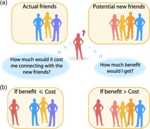
Consider individuals in a social network. Naturally, they wish to gain prominence by navigating the network and seeking strategic ties. The objective is not simply to pursue a large number of connections, but to obtain the right connections—ones that place the individual in a central network position. For example, seeking a junction that bridges between many pathways, and hence funnels much of the flow of information in the network.

Of course, such centrality in the network, while offering extremely valuable social capital, does not come for free. Friendship has a cost. It requires constant maintenance.

As a result, the research shows, social networks, whether on or offline, are a dynamic beehive of individuals constantly playing the cost-benefit game, severing connections on the one hand, and establishing new ones on the other. It’s a constant buzz driven by the ambition for social centrality. At the end, when this tug-of-war reaches an equilibrium, all individuals have secured their position in the network, a position that best balances between their drive for prominence and their limited budget for new friendships.

“When we did the math,” says Prof. Baruch Barzel, one of the paper’s lead authors, “we discovered an amazing result: this process always ends with social paths centered around the number six. This is quite surprising. We need to understand that each individual in the network acts independently, without any knowledge or intention about the network as a whole. But still, this self-driven game shapes the structure of the entire network. It leads to the small world phenomenon, and to the recurring pattern of six degrees,” adds Prof. Barzel.

The short paths characterizing social networks are not merely a curiosity. They are a defining feature of the network’s behaviour. Our ability to spread information, ideas and fads that sweep through society is deeply ingrained in the fact that it only requires a few hops to link between seemingly unrelated individuals.

Of course, not only do ideas spread through social connections. Viruses and other pathogens use them, as well. The grave consequences of this social connectedness were witnessed firsthand with the rapid spread of the COVID pandemic that demonstrated to us all the power of six degrees. Indeed, within six infection cycles, a virus can cross the globe.

“But on the upside,” adds Prof. Barzel, “this collaboration is a great example of how six degrees can play in our favour. How else would a team from six countries around the world come together? This is truly six degrees in action!”

For more such insights, log into our website https://international-maths-challenge.com

Credit of the article given to Bar-Ilan University

Shuffling a pack of cards isn’t as easy as you think, not if you want to truly randomise the cards. Most people will give a pack a few shuffles with the overhand or riffle methods (where the pack is split and the two halves are interweaved). But research has shown this isn’t enough to produce a sufficiently random order to make sure the card game being played is completely fair and to prevent people cheating.

As I wrote in a recent article about card counting, not having an effective shuffling mechanism can be a serious problem for casinos:

Players have used shuffle tracking, where blocks of cards are tracked so that you have some idea when they will appear. If you are given the option to cut the pack, you try and cut the pack near where you think the block of cards you are tracking is so that you can bet accordingly. A variant on this is to track aces as, if you know when one is likely to appear, you have a distinct advantage over the casino.

So how can you make sure your cards are well and truly shuffled?

To work out how many ways there are of arranging a standard 52-card deck, we multiply 52 by all the numbers that come before it (52 x 51 x 50 … 3 x 2 x 1). This is referred to as “52 factorial” and is usually written as “52!” by mathematicians. The answer is so big it’s easier to write it using scientific notation as 8.0658175e+67, which means it’s a number beginning with 8, followed by 67 more digits.

To put this into some sort of context, if you dealt one million hands of cards every second, it would take you 20 sexdecillion, or 20,000,000,000,000,000,000,000,000,000,000,000,000,000,000,000,000,000, years to deal the same number of hands as there are ways to arrange a deck of cards.

You would think that it would be easy to get a random order from that many permutations. In fact, every arrangement is, in a sense, random. Even one where the cards are ordered by suit and then rank could be considered random. It is only the interpretation we put on this order that would make most people not consider it random. This is the same as the idea that the lottery is less likely to throw up the numbers one to six, whereas in reality this combination is just as probable as any other.

In theory, you could shuffle a deck so that the cards emerged in number order (all the aces, followed by all the twos, followed by all the threes and so on), with each set of numbers in the same suit order (say spades, hearts, diamonds and clubs). Most people would not consider this random, but it is just as likely to appear as any other specific arrangement of cards (very unlikely). This is an extreme example but you could come up with an arrangement that would be seen as random when playing bridge because it offered the players no advantage, but wouldn’t be random for poker because it produced consistently strong hands.

But what would a casino consider random? Mathematicians have developed several ways of measuring how random something is. Variation distance and separation distance are two measures calculated by mathematical formulas. They have a value of 1 for a deck of cards in perfect order (sorted by numbers and suits) and lower values for more mixed arrangements. When the values are less than 0.5, the deck is considered randomly shuffled. More simply, if you can guess too many cards in a shuffled deck, then the deck is not well shuffled.

Persi Diaconis is a mathematician who has been studying card shuffling for over 25 years. Together with and Dave Bayer, he worked out that to produce a mathematically random pack, you need to use a riffle shuffle seven times if you’re using the variation distance measure, or 11 times using the separation distance. The overhand shuffle, by comparison, requires 10,000 shuffles to achieve randomness.

“The usual shuffling produces a card order that is far from random,” Diaconis has said. “Most people shuffle cards three or four times. Five times is considered excessive”.

But five is still lower than the number required for an effective shuffle. Even dealers in casinos rarely shuffle the required seven times. The situation is worse when more than one deck is used, as is the case in blackjack. If you are shuffling two decks, you should shuffle nine times and for six decks you need to shuffle twelve times.

Many casinos now use automatic shuffling machines. This not only speeds up the games but also means that shuffles can be more random, as the machines can shuffle for longer than the dealers. These shuffling machines also stop issues such as card counting and card tracking.

But even these machines are not enough. In another study, Diaconis and his colleagues were asked by a casino to look at a new design of a card shuffling machine that the casino had built. The researchers found that the machine was not sufficiently random, as they simply did not shuffle enough times. But using the machine twice would resolve the problem.

So next time you’re at a casino, take a look at how many times the dealers shuffle. The cards may not be as random as you think they are, which could be to your advantage.

For more insights like this, visit our website at www.international-maths-challenge.com.
Credit of the article given to Graham Kendall

How can parents best help their children with their schooling without actually doing it for them? This article is part of our series on Parents’ Role in Education, focusing on how best to support learning from early childhood to Year 12.

Before beginning official schooling, parents can give their young children a boost in learning mathematics by noticing, exploring and talking about maths during everyday activities at home or out and about.

New research shows that parents play a key role in helping their children learn mathematics concepts involving time, shape, measurement and number. This mathematical knowledge developed before school is predictive of literacy and numeracy achievements in later grades.

One successful approach for strengthening the role of parents in mathematics learning is Let’s Count, implemented by The Smith Family. This builds on parents’ strengths and capabilities as the first mathematics educators of their children.

The Let’s Count longitudinal evaluation findings show that when early years educators encourage parents and families to confidently notice, explore and talk about mathematics in everyday activities, their young children’s learning flourishes.

Indeed, children whose families had taken part in Let’s Count showed greater mathematical skills than those in a comparison group whose families had not participated. For example, they were more successful with correctly making a group of seven (89% versus 63%); continuing patterns (56% versus 34%); and counting collections of 20 objects (58% versus 37%).

These findings, among many others, are a strong endorsement of the power of families helping their children to learn about mathematics in everyday contexts.

What parents can do to promote maths every day

Discussing and exploring mathematics with children requires no special resources. Instead, what is needed is awareness and confidence for parents about how to engage.

However, our research shows that one of the biggest barriers to this is parents’ lack of confidence in leading maths education at home.

Through examining international research, we identified the type of activities that are important for early maths learning which are easy for parents to use. These include:

1. Comparing objects and describing which is longer, shorter, heavier, or holds less.
2. Playing with and describing 2D shapes and 3D objects.
3. Describing where things are positioned, for example, north, outside, behind, opposite.
4. Describing, copying, and extending patterns found in everyday situations.
5. Using time-words to describe points in time, events and routines (including days, months, seasons and celebrations).
6. Comparing and talking about the duration of everyday events and the sequence in which they occur.
7. Saying number names forward in sequence to ten (and eventually to 20 and beyond).
8. Using numbers to describe and compare collections.
9. Using perceptual and conceptual subitising (recognising quantities based on visual patterns), counting and matching to compare the number of items in one collection with another.
10. Showing different ways to make a total (at first with models and small numbers).
11. Matching number names, symbols and quantities up to ten.

Games to play using everyday situations

Neuroscience research has provided crucial evidence about the importance of early nurturing and support for learning, brain development, and the development of positive dispositions for learning.

Early brain development or “learning” is all about the quality of children’s sensory and motor experiences within positive and nurturing relationships and environments. This explains why programs such as Let’s Count are successful.

Sometimes it can be difficult to come up with activities and games to play that boost children’s mathematics learning, but there are plenty. For example, talk with your children as you prepare meals together. Talk about measuring and comparing ingredients and amounts.

You can play children’s card games and games involving dice, such as Snakes and Ladders, or maps, shapes and money. You can also read stories and notice the mathematics – the sequence of events, and the descriptions of characters and settings.

Although these activities may seem simple and informal, they build on what children notice and question, give families the chance to talk about mathematical ideas and language, and show children that maths is used throughout the day.

Parents are encouraged to provide learning opportunities that are engaging and relevant to their children. www.shutterstock.com

Make it relevant to them

Most importantly, encouraging maths and numeracy in young children relies on making it appealing and relevant to them.

For example, when you take your child for a walk down the street, in the park or on the beach, bring their attention to the objects around them – houses, cars, trees, signs.

Talk about the shapes and sizes of the objects, talk about and look for similarities and differences (for example: let’s find a taller tree or a heavier rock), count the number of cars parked in the street or time how long it takes to reach the next corner.

Discuss the temperature or the speed of your walking pace.

Collect leaves or shells, and make repeating patterns on the sand or grass, or play Mathematical I Spy (I spy with my little eye, something that’s taller than mum).

It is never too soon to begin these activities. Babies who are only weeks old notice differences in shapes and the number of objects in their line of sight.

So, from the earliest of ages, talk with your child about the world around them, being descriptive and using mathematical words. As they grow, build on what they notice about shapes, numbers, and measures. This is how you teach them mathematics.

For more insights like this, visit our website at www.international-maths-challenge.com.
Credit of the article given to Sivanes Phillipson, Ann Gervasoni

An artificial intelligence that can turn mathematical concepts written in English into a formal proving language for computers could make problems easier for other AIs to solve.

Maths can be difficult for a computer to understand

An artificial intelligence can translate maths problems written in plain English to formal code, making them easier for computers to solve in a crucial step towards building a machine capable of discovering new maths.

Computers have been used to verify mathematical proofs for some time, but they can only do it if the problems have been prepared in a specifically designed proving language, rather than for the mix of mathematical notation and written text used by mathematicians. This process, known as formalisation, can take years of work for just a single proof, so only a small fraction of mathematical knowledge has been formalised and then proved by a machine.

Yuhuai Wu at Google and his colleagues used a neural network called Codex created by AI research company OpenAI. It has been trained on large amounts of text and programming data from the web and can be used by programmers to generate workable code.

Proving languages share similarities with programming languages, so the team decided to see if Codex could formalise a bank of 12,500 secondary school maths competition problems. It was able to translate a quarter of all problems into a format that was compatible with a formal proof solver program called Isabelle. Many of the unsuccessful translations were the result of the system not understanding certain mathematical concepts, says Wu. “If you show the model with an example that explains that concept, the model can then quickly pick it up.”

To test the effectiveness of this auto-formalisation process, the team then applied Codex to a set of problems that had already been formalised by humans. Codex generated its own formal versions of these problems, and the team used another AI called MiniF2F to solve both versions.

The auto-formalised problems improved MiniF2F’s success rate from 29 per cent to 35 per cent, suggesting that Codex was better at formalising these problems than the humans were.

It is a modest improvement, but Wu says the team’s work is only a proof of concept. “If the goal is to train a machine that is capable of doing the same level of mathematics as the best humans, then auto-formalisation seems to be a very crucial path towards it,” says Wu.

Improving the success rate further would allow AIs to compete with human mathematicians, says team member Albert Jiang at the University of Cambridge. “If we get to 100 per cent, we will definitely be creating an artificial intelligence agent that’s able to win an International Maths Olympiad gold medal,” he says, referring to the top prize in a leading maths competition.

While the immediate goal is to improve the auto-formalisation models, and automated proving machines, there could be larger implications. Eventually, says Wu, the models could uncover areas of mathematics currently unknown to humans.

The capacity for reasoning in such a machine could also make it well-suited for verification tasks in a wide range of fields. “You can verify whether a piece of software is doing exactly what you asked it to do, or you can verify hardware chips, so it has applications in financial trading algorithms and hardware design,” says Jiang.

It is an exciting development for using machines to find new mathematics, says Yang-Hui He at the London Institute for Mathematical Sciences, but the real challenge will be in using the model on mathematical research, much of which is written in LaTeX, a typesetting system. “We only use LaTeX because it types nicely, but it’s a natural language in some sense, it has its own rules,” says He.

Users can define their own functions and symbols in LaTeX that might only be used in a single mathematical paper, which could be tricky for a neural network to tackle that has only been trained on the plain text, says He.

For more such insights, log into www.international-maths-challenge.com.

*Credit for article given to Alex Wilkins*

Credit: Can you find the center of a shape? You’ll be able to–even for the oddest oblong creation–with this simple science activity. No strings attached (okay, maybe one)!  George Retseck

A centering science activity

Introduction
With a little time, you can probably find the center of simple shapes such as circles and squares pretty easily. But how do you find the “middle” of an irregular shape such as a drawing of a dog or a cat? This project will show you how to do it using nothing but string and paper clips!

Background
How do you define the exact center of an object? One way to do this is to find the object’s center of mass. The center of mass is the point about which an object will balance if you try to rest it on your fingertip. Or if you hang an object, for example a picture frame from a nail, the center of mass will hang directly below the nail.

For symmetrical objects, finding the center of mass is relatively easy. For example, for a rectangular picture frame, you know the center of mass is in the middle of the rectangle and you can find that with a ruler. When you hang the picture frame, you will make sure it is centered on the nail—otherwise it will tip to one side and will be off-center. The same applies to other symmetrical objects such as a spherical basketball; you know the center of mass is in the middle of the sphere.

What about irregularly shaped objects such as a dog or cat or person? Now finding the center of mass is not so easy! This activity will show you how to find the center of mass for any two-dimensional shape you cut out of paper using a trick that has to do with the hanging picture frame mentioned above. If you hang a shape from a single point, you know the center of mass will always rest directly below that point. So, if you hang a shape from two different points (one at a time) and draw a line straight down from each point, the center of mass is where those lines intersect. This technique can be used for any irregular two-dimensional shape. Don’t believe it? Try this activity to find out!

Materials

• Paper (Heavier paper, such as construction paper, card stock or thin cardboard from the side of a cereal box will work best.)
• Scissors (Have an adult help with cutting if necessary—especially on thicker materials.)
• String
• Pencil
• Ruler
• Two paper clips or a pushpin and another small, relatively heavy object you can tie to the string (such as a metal washer)

Preparation

• Cut a piece of string about one foot long and tie a paper clip to each end. (Alternatively, you can use any other small object such as a metal washer on one end—this will serve as a weight—and any other small, pointy object like a needle or pushpin on the other end—this will be used to puncture the paper.)

Procedure

• Start with an easy shape: Cut out a rectangular piece of paper or cardboard. Can you guess where the center of mass of the rectangle is? If so, use a ruler to measure where you think it will be and mark this spot with your pencil.
• Punch several small holes around the edge of the paper. Make them as close to the edge as possible without ripping the paper. (This is important for the accuracy of this technique). The exact location of the holes does not matter but this technique will work best if you space them all the way around the edge (not just put two holes right next to each other).
• Now poke one end of one paper clip (or pushpin) through one of the holes to act like a hanging hook. Make sure the paper can swing easily from the hook and does not get stuck (Rotate it back and forth a few times to loosen the hole if necessary).
• Hold on to your “hook” and hold the paper up against the wall. Let the paper swing freely and make sure the string can hang straight down and does not get stuck.
• Use a pencil and ruler to draw a straight line on the paper along the string. Does this line go through the center of mass you predicted earlier?
• Now, hang your paper from a different hole and repeat the process. Where does this line intersect the first line?
• Repeat the process several more times with different holes. Do all the lines intersect at the same point?
• Now cut out an irregular shape. You can cut out a “blob” or draw something like a dog or cat and then cut out the outline. Make sure the shape you cut out remains stiff and flat. (That is, do not cut very thin sections that might be floppy.) Can you use a ruler to predict where the center of mass of your irregular shape will be? This is much harder!
• Punch holes around the edge of your irregular shape and repeat the activity. One at a time, hang the shape and the string from one of the holes and draw a line along the string. Where do the lines intersect? Does this match up with what you predicted?
• Extra: If you use a stiff enough material to cut out your shape (such as cardboard), can you try balancing it on your fingertip at the center of mass? What happens if you try to balance it about another point?

Observations and results
You should have found that the center of mass of the rectangle is right in the middle of the piece—halfway along the width and halfway along the height. You can easily locate this spot with a ruler. Then, when you hang the rectangle from a hole on its edge, the string should always pass through this point, regardless of which hole you use. Whereas it is much harder to predict the center of mass for an irregular shape, the same principle holds true.

Regardless of what point you hang the irregular shape from, the string will always pass through the center of mass. So, if you hang it from two or more points (one at a time), you can find the intersection of these lines—and that is the center of mass.

Note that due to small variables in the activity (such as friction on the hook that prevents the paper from rotating perfectly or the holes not being close enough to the edge of the paper), if you draw multiple lines, they might not all intersect in exactly the same place but they should still be fairly close to one another.

For more insights like this, visit our website at www.international-maths-challenge.com.

Credit of the article given to Ben Finio & Science Buddies

Credit: Heads or tails: Is it a 50-50 chance? Crunch some numbers and flip some coins to find out! George Retseck

A probabilistic science project from Science Buddies

Introduction
Have you ever heard anyone say the chance of something happening is “50–50”? What does that actually mean? This phrase has something to do with probability. Probability tells you how likely it is that an event will occur. This means that for certain events you can actually calculate how likely it is that they will happen. In this activity, you will do these calculations and then test them to see whether they hold true for reality!

Background
Probability allows us to quantify the likelihood an event will occur. You might be familiar with words we use to talk about probability, such as “certain,” “likely,” “unlikely,” “impossible,” and so on. You probably also know that the probability of an event happening spans from impossible, which means that this event will not happen under any circumstance, to certainty, which means that an event will happen without a doubt. In mathematics, these extreme probabilities are expressed as 0 (impossible) and 1 (certain). This means a probability number is always a number from 0 to 1. Probability can also be written as a percentage, which is a number from 0 to 100 percent. The higher the probability number or percentage of an event, the more likely is it that the event will occur.

The probability of a certain event occurring depends on how many possible outcomes the event has. If an event has only one possible outcome, the probability for this outcome is always 1 (or 100 percent). If there is more than one possible outcome, however, this changes. A simple example is the coin toss. If you toss a coin, there are two possible outcomes (heads or tails). As long as the coin was not manipulated, the theoretical probabilities of both outcomes are the same–they are equally probable. The sum of all possible outcomes is always 1 (or 100 percent) because it is certain that one of the possible outcomes will happen. This means that for the coin toss, the theoretical probability of either heads or tails is 0.5 (or 50 percent).

It gets more complicated with a six-sided die. In this case if you roll the die, there are 6 possible outcomes (1, 2, 3, 4, 5 or 6). Can you figure out what the theoretical probability for each number is? It is 1/6 or 0.17 (or 17 percent). In this activity, you will put your probability calculations to the test. The interesting part about probabilities is that knowing the theoretical likelihood of a certain outcome doesn’t necessarily tell you anything about the experimental probabilities when you actually try it out (except when the probability is 0 or 1). For example, outcomes with very low theoretical probabilities do actually occur in reality, although they are very unlikely. So how do your theoretical probabilities match your experimental results? You will find out by tossing a coin and rolling a die in this activity.

Materials

• Coin
• Six-sided die
• Paper
• Pen or pencil

Preparation

• Prepare a tally sheet to count how many times the coin has landed on heads or tails.
• Prepare a second tally sheet to count how often you have rolled each number with the die.

Procedure

• Calculate the theoretical probability for a coin to land on heads or tails, respectively. Write the probabilities in fraction form. What is the theoretical probability for each side? 
• Now get ready to toss your coin. Out of the 10 tosses, how often do you expect to get heads or tails?
• Toss the coin 10 times. After each toss, record if you got heads or tails in your tally sheet.
• Count how often you got heads and how often you got tails. Write your results in fraction form. For example, 3 tails out of 10 tosses would be 3/10 or 0.3. (The denominator will always be the number of times you toss the coin, and the numerator will be the outcome you are measuring, such as the number of times the coin lands on tails.) You could also express the same results looking at heads landings for the same 10 tosses. So that would be 7 heads out of 10 tosses: 7/10 or 0.7. Do your results match your expectations?
• Do another 10 coin tosses. Do you expect the same results? Why or why not?
• Compare your results from the second round with the ones from the first round. Are they the same? Why or why not?
• Continue tossing the coin. This time toss it 30 times in a row. Record your results for each toss in your tally sheet. What results do you expect this time?
• Look at your results from the 30 coin tosses and convert them into fraction form. How are they different from your previous results for the 10 coin tosses?
• Count how many heads and tails you got for your total coin tosses so far, which should be 50. Again, write your results in fraction form (with the number of tosses as the denominator (50) and the result you are tallying as the numerator). Does your experimental probability match your theoretical probability from the first step? (An easy way to convert this fraction into a percentage is to multiply the denominator and the numerator each by 2, so 50 x 2 = 100. And after you multiply your numerator by 2, you will have a number that is out of 100—and a percentage.)
• Calculate the theoretical probability for rolling each number on a six-sided die. Write the probabilities in fraction form. What is the theoretical probability for each number?
• Take the dice and roll it 10 times. After each roll, record which number you got in your tally sheet. Out of the 10 rolls, how often do you expect to get each number?
• After 10 rolls, compare your results (written in fraction form) with your predictions. How close are they?
• Do another 10 rolls with the dice, recording the result of each roll. Do your results change?
• Now roll the dice 30 times in a row (recording the result after each roll). How often did you roll each number this time?
• Count how often you rolled each number in all combined 50 rolls. Write your results in fraction form. Does your experimental probability match your theoretical probability? (Use the same formula you used for the coin toss, multiplying the denominator and the numerator each by 2 to get the percentage.)
• Compare your calculated probability numbers with your actual data for both activities (coin and dice). What do your combined results tell you about probability?
• Extra: Increase the number of coin tosses and dice rolls even further. How do your results compare with the calculated probabilities with increasing number of events (tosses or rolls)? 
• Extra: Look up how probabilities can be represented by probability trees. Can you draw a probability tree for the coin toss and dice roll?
• Extra: If you are interested in more advanced probability calculations, find out how you can calculate the probability of a recurring event, for example: How likely it is that you would get two heads in a row when tossing a coin? 

Observations and Results
Calculating the probabilities for tossing a coin is fairly straightforward. A coin toss has only two possible outcomes: heads or tails. Both outcomes are equally likely. This means that the theoretical probability to get either heads or tails is 0.5 (or 50 percent). The probabilities of all possible outcomes should add up to 1 (or 100 percent), which it does. When you tossed the coin 10 times, however, you most likely did not get five heads and five tails. In reality, your results might have been 4 heads and 6 tails (or another non-5-and-5 result). These numbers would be your experimental probabilities. In this example, they are 4 out of 10 (0.4) for heads and 6 out of 10 (0.6) for tails. When you repeated the 10 coin tosses, you probably ended up with a different result in the second round. The same was probably true for the 30 coin tosses. Even when you added up all 50 coin tosses, you most likely did not end up in a perfectly even probability for heads and tails. Your experimental probabilities thus probably didn’t match your calculated (theoretical) probabilities.

You likely observed a similar phenomenon when rolling the dice. Although the theoretical probability for each number is 1 out of 6 (1/6 or 0.17), in reality your experimental probabilities probably looked different. Instead of rolling each number 17 percent out of your total rolls, you might have rolled them more or less often.

If you continued tossing the coin or rolling the dice, you probably have observed that the more trials (coin tosses or dice rolls) you did, the closer the experimental probability was to the theoretical probability. Overall these results mean that even if you know the theoretical probabilities for each possible outcome, you can never know what the actual experimental probabilities will be if there is more than one outcome for an event. After all, a theoretical probability is just predicting how the chances are that an event or a specific outcome occurs—it won’t tell you what will actually happen!

For more insights like this, visit our website at www.international-maths-challenge.com.

Credit of the article given to Science Buddies & Svenja Lohner

There are some great uses. Shutterstock

Despite the fact that mathematics is often described as the underpinning science, it is often not given enough credit when scientific discoveries are presented. But the contribution of mathematics and statistics is essential and has transformed entire areas of research – many discoveries would not have been possible without it. In fact, as a mathematician, I have contributed to scientific discoveries and provided solutions to problems that biology was yet to solve.

Seven years ago, I attended a lecture on some biological research that was taking place at Heriot-Watt University. My colleagues had an unsolved problem which related to the movement of bag-like structures called vesicles which move hormones and neurotransmitters such as insulin or serotonin around cells and the body.

Their problem lay in that vesicles were known to follow specific tracks along the cell skeleton which lead to special molecules which then caused the vesicle to release its contents into the cell. However, when the biologists themselves tried to find these tracks, they were not in the expected places.

A bag that carries hormones to their location. OpenStax, CC BY

It is important to understand how vesicles behave, or in fact misbehave, as they have been linked to conditions such diabetes and neurological disorders. The biologists were struggling to find a way to understand the vesicles – but I had a solution in my mathematical toolkit.

Maths can beat biology

After two years of collaboration I told my colleagues: “my model and computer experiments are better than your microscope!”

What I meant by this rather confident statement was that by using mathematics to model how molecules move in a cell we could predict and run multiple experiments on a computer at a smaller scale and faster rate than a microscope. It could allow us to uncover things that the biologist’s resources could not, and might even point us in the direction of target molecules for future treatments of diabetes and neurological disorders.

The mathematical model allowed us to recognise that the movement of vesicles requires energy – and the maths models it through an energy landscape. It imagined a vesicle to be like a cyclist riding a bicycle – the landscape may have easy level sections but also hills that require more energy input to get over them, and so we wanted to test whether they actually avoided these hills.

After seven years of working in partnership with the biologists, my colleagues and I proved our hypothesis was correct. Vesicles do follow lower energy “valleys” in the landscape, avoiding molecules which create the high energy hills in the energy landscape – taking the easiest path. The overall result is just the same as the biologists had found – the vesicles end up in the same end location and they reuse similar routes over and over again. But the difference lies in the way in which they do it, and it was not by following the cell skeleton as biologists had first believed – they take an easier route. It really shows the power of maths and how it can change the way we see things.

Mathematical models allow you to capture many gigabytes of raw data in a compact form in a way that is impossible for a biologist with a microscope. You can make modifications to the model easily and show how vesicle behaviour may change during disease, when they are disrupted or mutated. It could then reveal which molecules to target in future treatment studies – and lay the groundwork for larger and more thorough modelling of complex biological processes.

A modelled energy landscape. Shutterstock

The integration of cutting-edge microscopy with cell biology and mathematical modelling could be applied to many other problems in bio-medicine and will accelerate discovery in the years to come. The movement of molecules and other cell components is just one example of where the power of mathematics is unrivalled, but it is by no means its limit.

Useful is an understatement

Maths is often criticised by the public for lacking in “real-world” applications, but it is being applied to many real-world problems all the time. Groundwater contamination, financial and economic forecasting, plume heights in volcanic eruptions, the modelling of biological processes and drug delivery are just a few places where maths is making a huge difference.

I’m proud to say that I co-authored a paper with my biology colleagues, and I hope to see more mathematicians coming to the fore for science research in the future. Mathematics plays a central role in so many of the world’s scientific breakthroughs and deserves a headline role in more academic publications. Power to the mathematician – they’re behind more discoveries than you think.

For more insights like this, visit our website at www.international-maths-challenge.com.
Credit of the article given to Gabriel Lord

A small dot on an old piece of birch bark marks one of the biggest events in the history of mathematics. The bark is actually part of an ancient Indian mathematical document known as the Bakhshali manuscript. And the dot is the first known recorded use of the number zero. What’s more, researchers from the University of Oxford recently discovered the document is 500 years older than was previously estimated, dating to the third or fourth century – a breakthrough discovery.

Today, it’s difficult to imagine how you could have mathematics without zero. In a positional number system, such as the decimal system we use now, the location of a digit is really important. Indeed, the real difference between 100 and 1,000,000 is where the digit 1 is located, with the symbol 0 serving as a punctuation mark.

Yet for thousands of years we did without it. The Sumerians of 5,000BC employed a positional system but without a 0. In some rudimentary form, a symbol or a space was used to distinguish between, for example, 204 and 20000004. But that symbol was never used at the end of a number, so the difference between 5 and 500 had to be determined by context.

What’s more, 0 at the end of a number makes multiplying and dividing by 10 easy, as it does with adding numbers like 9 and 1 together. The invention of zero immensely simplified computations, freeing mathematicians to develop vital mathematical disciplines such as algebra and calculus, and eventually the basis for computers.

Zero’s late arrival was partly a reflection of the negative views some cultures held for the concept of nothing. Western philosophy is plagued with grave misconceptions about nothingness and the mystical powers of language. The fifth century BC Greek thinker Parmenides proclaimed that nothing cannot exist, since to speak of something is to speak of something that exists. This Parmenidean approach kept prominent historical figures busy for a long while.

After the advent of Christianity, religious leaders in Europe argued that since God is in everything that exists, anything that represents nothing must be satanic. In an attempt to save humanity from the devil, they promptly banished zero from existence, though merchants continued secretly to use it.

By contrast, in Buddhism the concept of nothingness is not only devoid of any demonic possessions but is actually a central idea worthy of much study en route to nirvana. With such a mindset, having a mathematical representation for nothing was, well, nothing to fret over. In fact, the English word “zero” is originally derived from the Hindi “sunyata”, which means nothingness and is a central concept in Buddhism.

The Bakhshali manuscript. Bodleian Libraries

So after zero finally emerged in ancient India, it took almost 1,000 years to set root in Europe, much longer than in China or the Middle East. In 1200 AD, the Italian mathematician Fibonacci, who brought the decimal system to Europe, wrote that:

The method of the Indians surpasses any known method to compute. It’s a marvellous method. They do their computations using nine figures and the symbol zero.

This superior method of computation, clearly reminiscent of our modern one, freed mathematicians from tediously simple calculations, and enabled them to tackle more complicated problems and study the general properties of numbers. For example, it led to the work of the seventh century Indian mathematician and astronomer Brahmagupta, considered to be the beginning of modern algebra.

Algorithms and calculus

The Indian method is so powerful because it means you can draw up simple rules for doing calculations. Just imagine trying to explain long addition without a symbol for zero. There would be too many exceptions to any rule. The ninth century Persian mathematician Al-Khwarizmi was the first to meticulously note and exploit these arithmetic instructions, which would eventually make the abacus obsolete.

Such mechanical sets of instructions illustrated that portions of mathematics could be automated. And this would eventually lead to the development of modern computers. In fact, the word “algorithm” to describe a set of simple instructions is derived from the name “Al-Khwarizmi”.

The invention of zero also created a new, more accurate way to describe fractions. Adding zeros at the end of a number increases its magnitude, with the help of a decimal point, adding zeros at the beginning decreases its magnitude. Placing infinitely many digits to the right of the decimal point corresponds to infinite precision. That kind of precision was exactly what 17th century thinkers Isaac Newton and Gottfried Leibniz needed to develop calculus, the study of continuous change.

And so algebra, algorithms, and calculus, three pillars of modern mathematics, are all the result of a notation for nothing. Mathematics is a science of invisible entities that we can only understand by writing them down. India, by adding zero to the positional number system, unleashed the true power of numbers, advancing mathematics from infancy to adolescence, and from rudimentary toward its current sophistication.

For more insights like this, visit our website at www.international-maths-challenge.com.
Credit of the article given to Ittay Weiss

Credit: Monty Rakusen Getty Images

Scientists have created a “map” of odor molecules, which could ultimately be used to predict new scent combinations 

The human nose finds it simple to distinguish the aroma of fresh coffee from the stink of rotten eggs, but the underlying biochemistry is complicated. Researchers have now created an olfactory “map”—a geometric model of how molecules combine to produce various scents. This map could inspire a way to predict how people might perceive certain odor combinations and help to drive the development of new fragrances, scientists say.

Researchers have been trying for years to tame the elaborate landscape of odor molecules. Neuroscientists want to better understand how we process scents; perfume and food manufacturers want better ways to synthesize familiar aromas for their products. The new approach may appeal to both camps.

One earlier strategy for mapping the olfactory system involves grouping odor molecules that have similar molecular structures and using those similarities to predict the scents of novel combinations. But that avenue often leads to a dead end. “It’s not necessary that chemicals with the same chemical structures will be perceived similarly,” says Tatyana Sharpee, a neurobiologist at the Salk Institute for Biological Studies in La Jolla, Calif., and lead author of the study, which appeared in August in Science Advances.

Sharpee and her colleagues analyzed odor molecules found in four familiar and unmistakable scents: strawberries, tomatoes, blueberries and mouse urine. The researchers calculated how often and in what concentrations certain molecules turned up together in these scents. They then created a mathematical model in which molecules that occurred together frequently were represented as closer in space and molecules that rarely did so were farther apart. The result was a “saddle”-shaped surface—a hallmark of a field called hyperbolic geometry, which obeys different rules from the geometry most people learn in school.

The researchers envision an algorithm, trained on this hyperbolic geometry model, that can predict the scents of new odor combinations—or even help to synthesize them. One of Sharpee’s collaborators, behavioral neuroscientist Brian Smith of Arizona State University, wants to use this method to create olfactory environments in places devoid of natural scents.

Such a tool would be useful to scientists and odor manufacturers alike, says olfactory neuroscientist Joel Mainland of the Monell Chemical Senses Center in Philadelphia, who was not involved in the study. The ultimate goal is to know enough about how odors work to replicate natural smells without the natural sources, Mainland says: “We want to identify a strawberry flavor without worrying about replicating the ingredients that are in a strawberry.”

For more insights like this, visit our website at www.international-maths-challenge.com.

Credit of the article given to Stephen Ornes