Category: mathematics

Credit: Getty Images

The right mix of people who already know one another, of boys and girls–Ramsey numbers may hold the answer

Let’s say you’re planning your next party and agonizing over the guest list. To whom should you send invitations? What combination of friends and strangers is the right mix?

It turns out mathematicians have been working on a version of this problem for nearly a century. Depending on what you want, the answer can be complicated.

Our book, “The Fascinating World of Graph Theory,” explores puzzles like these and shows how they can be solved through graphs. A question like this one might seem small, but it’s a beautiful demonstration of how graphs can be used to solve mathematical problems in such diverse fields as the sciences, communication and society.

A puzzle is born

While it’s well-known that Harvard is one of the top academic universities in the country, you might be surprised to learn that there was a time when Harvard had one of the nation’s best football teams. But in 1931, led by All–American quarterback Barry Wood, such was the case.

That season Harvard played Army. At halftime, unexpectedly, Army led Harvard 13–0. Clearly upset, Harvard’s president told Army’s commandant of cadets that while Army may be better than Harvard in football, Harvard was superior in a more scholarly competition.

Though Harvard came back to defeat Army 14-13, the commandant accepted the challenge to compete against Harvard in something more scholarly. It was agreed that the two would compete – in mathematics. This led to Army and Harvard selecting mathematics teams; the showdown occurred in West Point in 1933. To Harvard’s surprise, Army won.

The Harvard–Army competition eventually led to an annual mathematics competition for undergraduates in 1938, called the Putnam exam, named for William Lowell Putnam, a relative of Harvard’s president. This exam was designed to stimulate a healthy rivalry in mathematics in the United States and Canada. Over the years and continuing to this day, this exam has contained many interesting and often challenging problems – including the one we describe above.

Red and blue lines

The 1953 exam contained the following problem (reworded a bit): There are six points in the plane. Every point is connected to every other point by a line that’s either blue or red. Show that there are three of these points between which only lines of the same color are drawn.

In math, if there is a collection of points with lines drawn between some pairs of points, that structure is called a graph. The study of these graphs is called graph theory. In graph theory, however, the points are called vertices and the lines are called edges.

Graphs can be used to represent a wide variety of situations. For example, in this Putnam problem, a point can represent a person, a red line can mean the people are friends and a blue line means that they are strangers.

Show that there are three points connected by lines of the same color. Credit: richtom80 Wikimedia (CC BY-SA 3.0)

For example, let’s call the points A, B, C, D, E, F and select one of them, say A. Of the five lines drawn from A to the other five points, there must be three lines of the same color.

Say the lines from A to B, C, D are all red. If a line between any two of B, C, D is red, then there are three points with only red lines between them. If no line between any two of B, C, D is red, then they are all blue.

What if there were only five points? There may not be three points where all lines between them are colored the same. For example, the lines A–B, B–C, C–D, D–E, E–A may be red, with the others blue.

From what we saw, then, the smallest number of people who can be invited to a party (where every two people are either friends or strangers) such that there are three mutual friends or three mutual strangers is six.

What if we would like four people to be mutual friends or mutual strangers? What is the smallest number of people we must invite to a party to be certain of this? This question has been answered. It’s 18.

What if we would like five people to be mutual friends or mutual strangers? In this situation, the smallest number of people to invite to a party to be guaranteed of this is – unknown. Nobody knows. While this problem is easy to describe and perhaps sounds rather simple, it is notoriously difficult.

Ramsey numbers

What we have been discussing is a type of number in graph theory called a Ramsey number. These numbers are named for the British philosopher, economist and mathematician Frank Plumpton Ramsey.

Ramsey died at the age of 26 but obtained at his very early age a very curious theorem in mathematics, which gave rise to our question here. Say we have another plane full of points connected by red and blue lines. We pick two positive integers, named r and s. We want to have exactly r points where all lines between them are red or s points where all lines between them are blue. What’s the smallest number of points we can do this with? That’s called a Ramsey number.

For example, say we want our plane to have at least three points connected by all red lines and three points connected by all blue lines. The Ramsey number – the smallest number of points we need to make this happen – is six.

When mathematicians look at a problem, they often ask themselves: Does this suggest another question? This is what has happened with Ramsey numbers – and party problems.

For example, here’s one: Five girls are planning a party. They have decided to invite some boys to the party, whether they know the boys or not. How many boys do they need to invite to be certain that there will always be three boys among them such that three of the five girls are either friends with all three boys or are not acquainted with all three boys? It’s probably not easy to make a good guess at the answer. It’s 41!

Very few Ramsey numbers are known. However, this doesn’t stop mathematicians from trying to solve such problems. Often, failing to solve one problem can lead to an even more interesting problem. Such is the life of a mathematician.

This article was originally published on The Conversation. Read the original article.

For more insights like this, visit our website at www.international-maths-challenge.com.

Credit of the article given to Gary Chartrand, Arthur Benjamin, Ping Zhang & The Conversation US

Abstract algebra class gave me the kick in the rear I needed to focus on the relationships between notes

During my senior year of college, I decided I wanted to expand my musical horizons, so I joined the early music ensemble. I had entered college with a viola scholarship, so I had played in the orchestra throughout my time there as well as doing chamber music and working on solo viola pieces, but I had always enjoyed early music and wanted to try something new. In the ensemble, I played Baroque violin, and a lot of my technique as a modern violist translated well. I held the instrument and bow a little differently, but on the whole, I was able to pick it up quickly. Reading the music was another story.

Many people are exposed to treble and bass clefs in music classes. I was very young when my mom started to teach me how to read music, but I still remember the feeling of accomplishment I had when I mastered the idea that the position of a spot on an array of lines and spaces corresponded to a particular key on a piano or a particular pitch I could sing. The treble clef is based on the G above middle C. The bass clef uses the F below middle C.

A C major scale written across bass (bottom) and treble (top) clefs. The two dots on the bass clef indicate the F below middle C, and the treble clef circles the G above middle C. Credit: Martin Marte-Singer Wikimedia (CC BY-SA 4.0)

Many instruments’ ranges fit comfortably onto either the treble or bass clef, perhaps adjusted by an octave when necessary. Piano music, of course, uses both clefs. But the viola is a little too low to use treble clef all the time and a little too high to use bass clef all the time. When I started to play viola, I learned to read alto clef, which has middle C smack dab in the middle of the staff, and eventually I was the music-reading equivalent of trilingual.

A C major scale written in alto clef, starting on middle C. Credit: Hyacinth Wikimedia

My multilingualism had its limits, though. I could read all three clefs, but if I wanted to play music originally written for cello an octave higher or music originally written for flute or violin an octave lower—tasks that would have been trivial on a piano—I would struggle to read bass clef up an octave or treble clef down an octave, respectively. Tenor clef, which is like alto clef but with the C one line higher, flummoxed me entirely. I wasn’t as fluent as I wanted to be.

Early music ensemble pushed my limits. Music from the Baroque era and before was not always notated using the small number of clefs we tend to use now. I was reading music in French violin clef (ooh-la-la, this one looks like treble clef but has the G on the bottom line instead of the line above the bottom), soprano clef (a C clef like alto and tenor clefs with the C on the bottom line), and other currently unusual clefs. It was overwhelming. I made a lot of mistakes in rehearsal, despite the many note names I had to write in my music.

The same semester I started playing with the early music ensemble, I took an abstract algebra class. Abstract algebra looks at structures of sets of numbers and symmetries. It encourages people to see connections between sometimes very different mathematical objects and transformations and to view the relationships between objects as fundamental to understanding those objects.

At some point in the semester, a switch flipped in my brain, and my early music clef struggles virtually disappeared. At the beginning of a piece, I would look at the clef to get my bearings, and I could see the rest of the notes as representing relationships between one pitch and the next. I read intervals, not pitches. I was not perfect, but I felt like almost overnight I had unlocked a new music-reading level.

I have always felt like my journey into more abstract algebra and my new clef fluency were related, but I have struggled to put that connection into words. I feel like the structural and relational aspects of abstract algebra helped me to see clefs as descriptions of relationships between notes rather than as absolute pitches, but I can’t point to a particular theorem or insight in abstract algebra that would apply explicitly.

Last year, I learned about the Yoneda lemma, an important theorem in the mathematical field of category theory. (According to our My Favorite Theorem guest Emily Riehl, it’s every category theorist’s favorite theorem.) I am no category theorist, but I found Tai-Danae Bradley’s description of the Yoneda lemma helpful, particularly the big idea she shared in this post on the Yoneda perspective. She writes that the punchline of the Yoneda lemma, or at least two of its corollaries, is “mathematical objects are completely determined by their relationships to other objects.”

It has taken me a while to make the connection explicitly, but I think the “Yoneda perspective” describes the mental shift I made in early music ensemble. It’s not the exact notes that matter when you’re reading music written in an unfamiliar clef but the relationships between them. Since having this shift in perspective, it’s been easier for me to transpose music into different keys and read treble and bass clefs in whatever octaves I need to.

Some organists and pianists can transpose music seemingly effortlessly to accommodate the needs of their church choirs or musical theater performers, and I think it’s because they’ve already shifted to the Yoneda perspective, even if that’s not how they would describe it. They didn’t necessarily get there via advanced mathematics classes, but for me, I think abstract algebra class gave me the kick in the rear I needed not to be tied to any one set of exact pitches but to focus on the relationships between them. I won’t claim that studying abstract algebra or category theory will improve your music-reading skills—making music, not studying a math book, is usually the best way to get better at making music—but pondering these connections enriches my experience of both math and music, and I hope it can do the same for you.

For more insights like this, visit our website at www.international-maths-challenge.com.

Credit of the article given to Evelyn Lamb

Credit: Getty Images

Processing high-level math concepts uses the same neural networks as the basic math skills a child is born with

Alan Turing, Albert Einstein, Stephen Hawking, John Nash—these “beautiful” minds never fail to enchant the public, but they also remain somewhat elusive. How do some people progress from being able to perform basic arithmetic to grasping advanced mathematical concepts and thinking at levels of abstraction that baffle the rest of the population? Neuroscience has now begun to pin down whether the brain of a math wiz somehow takes conceptual thinking to another level.

Specifically, scientists have long debated whether the basis of high-level mathematical thought is tied to the brain’s language-processing centers—that thinking at such a level of abstraction requires linguistic representation and an understanding of syntax—or to independent regions associated with number and spatial reasoning. In a study published this week in Proceedings of the National Academy of Sciences, a pair of researchers at the INSERM–CEA Cognitive Neuroimaging Unit in France reported that the brain areas involved in math are different from those engaged in equally complex nonmathematical thinking.

The team used functional magnetic resonance imaging (fMRI) to scan the brains of 15 professional mathematicians and 15 nonmathematicians of the same academic standing. While in the scanner the subjects listened to a series of 72 high-level mathematical statements, divided evenly among algebra, analysis, geometry and topology, as well as 18 high-level nonmathematical (mostly historical) statements. They had four seconds to reflect on each proposition and determine whether it was true, false or meaningless.

The researchers found that in the mathematicians only, listening to math-related statements activated a network involving bilateral intraparietal, dorsal prefrontal, and inferior temporal regions of the brain. This circuitry is usually not associated with areas involved in language processing and semantics, which were activated in both mathematicians and nonmathematicians when they were presented with the nonmathematical statements. “On the contrary,” says study co-author and graduate student Marie Amalric, “our results show that high-level mathematical reflection recycles brain regions associated with an evolutionarily ancient knowledge of number and space.”

Previous research has found that these nonlinguistic areas are active when performing rudimentary arithmetic calculations and even simply seeing numbers on a page, suggesting a link between advanced and basic mathematical thinking. In fact, co-author Stanislas Dehaene, director of the Cognitive Neuroimaging Unit and experimental psychologist, has studied how humans (and even some animal species) are born with an intuitive sense of numbers—of quantity and arithmetic manipulation—closely related to spatial representation. How the connection between a hardwired “number sense” and higher-level math is formed, however, remains unknown. This work raises the intriguing question of whether an innate capability to recognize different quantities—that two pieces of fruit are greater than one—is the biological foundation on which can be built the capacity to master group theory. “It would be interesting to investigate the causal chain between lower-level and higher-level mathematical competency,” says Daniel Ansari, a cognitive neuroscientist at the University of Western Ontario who did not participate in the study. “Most of us master basic arithmetic, so we’re already recruiting these brain regions, but only a fraction of us go on to do high-level math. We don’t yet know whether becoming a mathematical expert changes the way you do arithmetic or whether learning arithmetic lays out the foundation for acquiring higher-level mathematical concepts.”

Ansari suggests that a training study, in which nonmathematicians are taught advanced mathematical concepts, could provide a better understanding of these connections and how they form. Moreover, achieving expertise in mathematics may affect neuronal circuitry in other ways. Amalric’s study found that mathematicians had reduced activity in the visual areas of the brain involved in facial processing. This could mean that the neural resources required to grasp and work with certain math concepts may undercut—or “use up”—some of the brain’s other capacities. Although additional studies are needed to determine whether mathematicians actually do process faces differently, the researchers hope to gain further insight into the effects that expertise has on how the brain is organized.

“We can start to investigate where exceptional abilities come from, and the neurobiological correlates of such high-level expertise,” Ansari says. “I just think it’s great that we now have the capability to use brain imaging to answer these deep questions about the complexity of human abilities.”

For more insights like this, visit our website at www.international-maths-challenge.com.

Credit of the article given to  Jordana Cepelewicz

Credit: Jasmina81 Getty Images

Why do Americans have such trouble with fractions—and what can be done?

Many children never master fractions. When asked whether 12/13 + 7/8 was closest to 1, 2, 19, or 21, only 24% of a nationally representative sample of more than 20,000 US 8th graders answered correctly. This test was given almost 40 years ago, which gave Hugo Lortie-Forgues and me hope that the work of innumerable teachers, mathematics coaches, researchers, and government commissions had made a positive difference. Our hopes were dashed by the data, though; we found that in all of those years, accuracy on the same problem improved only from 24% to 27% correct.

Such difficulties are not limited to fraction estimation problems nor do they end in 8th grade. On standard fraction addition, subtraction, multiplication, and division problems with equal denominators (e.g., 3/5+4/5) and unequal denominators (e.g., 3/5+2/3), 6th and 8th graders tend to answer correctly only about 50% of items. Studies of community college students have revealed similarly poor fraction arithmetic performance. Children in the US do much worse on such problems than their peers in European countries, such as Belgium and Germany, and in Asian countries such as China and Korea.

This weak knowledge is especially unfortunate because fractions are foundational to many more advanced areas of mathematics and science. Fifth graders’ fraction knowledge predicts high school students’ algebra learning and overall math achievement, even after controlling for whole number knowledge, the students’ IQ, and their families’ education and income. On the reference sheets for recent high school AP tests in chemistry and physics, fractions were part of more than half of the formulas. In a recent survey of 2300 white collar, blue collar, and service workers, more than two-thirds indicated that they used fractions in their work. Moreover, in a nationally representative sample of 1,000 Algebra 1 teachers in the US, most rated as “poor” their students’ knowledge of fractions and rated fractions as the second greatest impediment to their students mastering algebra (second only to “word problems”).

Why are fractions so difficult to understand? A major reason is that learning fractions requires overcoming two types of difficulty: inherent and culturally contingent. Inherent sources of difficulty are those that derive from the nature of fractions, ones that confront all learners in all places. One inherent difficulty is the notation used to express fractions. Understanding the relation a/b is more difficult than understanding the simple quantity a, regardless of the culture or time period in which a child lives. Another inherent difficulty involves the complex relations between fraction arithmetic and whole number arithmetic. For example, multiplying fractions involves applying the whole number operation independently to the numerator and the denominator (e.g., 3/7 * 2/7 = (3*2)/(7*7) = 6/49), but doing the same leads to wrong answers on fraction addition (e.g., 3/7 + 2/7 ≠ 5/14). A third inherent source of difficulty is complex conceptual relations among different fraction arithmetic operations, at least using standard algorithms. Why do we need equal denominators to add and subtract fractions but not to multiply and divide them? Why do we invert and multiply to solve fraction division problems, and why do we invert the fraction in the denominator rather than the one in the numerator? These inherent sources of difficulty make understanding fraction arithmetic challenging for all students.

Culturally contingent sources of difficulty, in contrast, can mitigate or exacerbate the inherent challenges of learning fractions. Teacher understanding is one culturally-contingent variable: When asked to explain the meaning of fraction division problems, few US teachers can provide any explanation, whereas the large majority of Chinese teachers provide at least one good explanation. Language is another culturally-contingent factor; East Asian languages express fractions such as 3/4 as “out of four, three,” which makes it easier to understand their meaning than relatively opaque terms such as “three fourth.” A third such variable is textbooks. Despite division being the most difficult operation to understand, US textbooks present far fewer problems with fraction division than fraction multiplication; the opposite is true in Chinese and Korean textbooks. Probably most fundamental are cultural attitudes: Math learning is viewed as crucial throughout East Asia, but US attitudes about its importance are far more variable.

Given the importance of fractions in and out of school, the extensive evidence that many children and adults do not understand them, and the inherent difficulty of the topic, what is to be done? Considering culturally contingent factors points to several potentially useful steps. Inculcating a deeper understanding of fractions among teachers will likely help them to teach more effectively. Explaining the meaning of fractions to students using clear language (for example, explaining that 3/4 means 3 of the 1/4 units), and requesting textbook writers to include more challenging problems are other promising strategies. Addressing inherent sources of difficulty in fraction arithmetic, in particular understanding of fraction magnitudes, can also make a large difference.

Fraction Face-off!, a 12-week program designed by Lynn Fuchs to help children from low-income backgrounds improve their fraction knowledge, seems especially promising. The program teaches children about fraction magnitudes through tasks such as comparing and ordering fraction magnitudes and locating fractions on number lines. After participating in Fraction Face-off!, fourth graders’ fraction addition and subtraction accuracy consistently exceeds of children receiving the standard classroom curriculum. This finding was especially striking because Fraction Face-off! devoted less time to explicit instruction in fraction arithmetic procedures than did the standard curriculum. Similarly encouraging findings have been found for other interventions that emphasize the importance of fraction magnitudes. Such programs may help children learn fraction arithmetic by encouraging them to note that answers such as 1/3+1/2 = 2/5 cannot be right, because the sum is less than one of the numbers being added, and therefore to try procedures that generate more plausible answers. These innovative curricula seem well worth testing on a wider basis.

For more insights like this, visit our website at www.international-maths-challenge.com.

Credit of the article given to Robert S. Siegler

Credit: Pavel Bolotov/Thinkstock (MARS)

A rare appearance by enigmatic Shinichi Mochizuki brings faint optimism about his famously impenetrable work

Nearly four years after Shinichi Mochizuki unveiled an imposing set of papers that could revolutionize the theory of numbers, other mathematicians have yet to understand his work or agree on its validity — although they have made modest progress.

Some four dozen mathematicians converged last week for a rare opportunity to hear Mochizuki present his own work at a conference on his home turf, Kyoto University’s Research Institute for Mathematical Sciences (RIMS).

Mochizuki is “less isolated than he was before the process got started”, says Kiran Kedlaya, a number theorist at the University of California, San Diego. Although at first Mochizuki’s papers, which stretch over more than 500 pages, seemed like an impenetrable jungle of formulae, experts have slowly discerned a strategy in the proof that the papers describe, and have been able to zero in on particular passages that seem crucial, he says.

And Jeffrey Lagarias, a number theorist at the University of Michigan in Ann Arbor, says that he got far enough to see that Mochizuki’s work is worth the effort. “It has some revolutionary new ideas,” he says.

Still, Kedlaya says that the more he delves into the proof, the longer he thinks it will take to reach a consensus on whether it is correct. He used to think that the issue would be resolved perhaps by 2017. “Now I’m thinking at least three years from now.”

Others are even less optimistic. “The constructions are generally clear, and many of the arguments could be followed to some extent, but the overarching strategy remains totally elusive for me,” says mathematician Vesselin Dimitrov of Yale University in New Haven, Connecticut. “Add to this the heavy, unprecedentedly indigestible notation: these papers are unlike anything that has ever appeared in the mathematical literature.”

The abc proof

Mochizuki’s theorem aims to prove the important abc conjecture, which dates back to 1985 and relates to prime numbers — whole numbers that cannot be evenly divided by any smaller number except by 1. The conjecture comes in a number of different forms, but explains how the primes that divide two numbers, a and b, are related to those that divide their sum, c.

If Mochizuki’s proof is correct, it would have repercussions across the entire field, says Dimitrov. “When you work in number theory, you cannot ignore the abc conjecture,” he says. “This is why all number theorists eagerly wanted to know about Mochizuki’s approach.” For example, Dimitrov showed in January how, assuming the correctness of Mochizuki’s proof, one might be able to derive many other important results, including a completely independent proof of the celebrated Fermat’s last theorem.

But the purported proof, which Mochizuki first posted on his webpage in August 2012, builds on more than a decade of previous work in which Mochizuki worked in virtual isolation and developed a novel and extremely abstract branch of mathematics.

Mochizuki in the room

The Kyoto workshop followed on the heels of one held last December in Oxford, UK. Mochizuki did not attend that first meeting, although he answered the audience’s questions over a Skype video link. This time, having him in the room — and hearing him present some of the materials himself — was helpful, says Taylor Dupuy, a mathematician at the Hebrew University of Jerusalem who participated in both workshops.

There are now around ten mathematicians who are putting substantial effort into digesting the material — up from just three before the Oxford workshop, says Ivan Fesenko, a mathematician at the University of Nottingham, UK, who co-organized both workshops. The group includes younger researchers, such as Dupuy.

In keeping with his reputation for being a very private person, Mochizuki — who is said to never eat meals in the presence of colleagues — did not take part in the customary mingling and social activities at the Kyoto meeting, according to several sources. And although he was unfailingly forthcoming in answering questions, it was unclear what he thought of the proceedings. “Mochizuki does not give a lot away,” Kedlaya says. “He’s an excellent poker player.”

Fellow mathematicians have criticized Mochizuki for his refusal to travel. After he posted his papers, he turned down multiple offers to spend time abroad and lecture on his ideas. Although he spent much of his youth in the United States, he is now said to rarely leave the Kyoto area. (Mochizuki does not respond to requests for interviews, and the workshop’s website contained the notice: “Activities aimed at interviewing or media coverage of any sort within the facilities of RIMS, Kyoto University, will not be accepted.”)

“He is very level-headed,” says another workshop participant, who did not want to be named. “The only thing that frustrates him is people making rash judgemental comments without understanding any details.”

Still, Dupuy says, “I think he does take a lot of the criticism about him really personally. I’m sure he’s sick of this whole thing, too.”

For more insights like this, visit our website at www.international-maths-challenge.com.

Credit of the article given to Davide Castelvecchi & Nature magazine

Credit: Ada Lovelace, Julia Robinson, and Emmy Noether. IanDagnall Computing/Alamy Stock Photo (Lovelace and Noether); George M. Bergman/Wikimedia Commons (CC BY-SA 4.0) (Robinson)

Everyone knows that history’s great mathematicians were all men—but everybody is wrong

This article was published in Scientific American’s former blog network and reflects the views of the author, not necessarily those of Scientific American

From the profound revelations of the shape of space to the furthest explorations reachable by imagination and logic, the history of mathematics has always been seen as a masculine endeavor. Names like Gauss, Euler, Riemann, Poincare, Erdős, and the more modern Wiles, Tao, Perelman, and Zhang, all of them associated with the most beautiful mathematics discovered since the dawn of humanity, are all men. The book Men of Mathematics, written by E.T. Bell in 1937, is just one example of how this “fact” has been reinforced in in the public consciousness.

Even today, it is no secret that male mathematicians still dominate the field. But this should not distract us from the revolutionary contributions women have made. We have notable women to thank for modern computation, revelations on the geometry of space, cornerstones of abstract algebra, and major advances in decision theory, number theory, and celestial mechanics that continue to provide crucial breakthroughs in applied areas like cryptography, computer science, and physics.

The works of geniuses like Julia Robinson on Hilbert’s Tenth Problem in number theory, Emmy Noether in abstract algebra and physics, and Ada Lovelace in computer science, are just three examples of women whose contributions have been absolutely essential.

Julia Robinson at Berkeley, California, 1975. Credit: George M. Bergman/Wikimedia Commons (CC BY-SA 4.0)

Julia Robinson (1919-1985)

At the turn of the twentieth century the famed German mathematician David Hilbert published a set of twenty-three tantalizing problems that had evaded the most brilliant of mathematical minds. Among them was his tenth problem, which asked if a general algorithm could be constructed to determine the solvability of any Diophantine equation (those polynomial equations with only integer coefficients and integer solutions). Imagine, for any Diophantine equation of the infinite set of such equations a machine that can tell whether it can be solved. Mathematicians often deal with infinite questions of this nature that exist far beyond resolution by simple extensive observations. This particular problem drew the attention of a Berkeley mathematician named Julia Robinson. Over several decades, Robinson collaborated with colleagues including Martin Davis and Hillary Putnam that resulted in formulating a condition that would answer Hilbert’s question in the negative.

In 1970 a young Russian mathematician named Yuri Matiyasevich solved the problem using the insight provided by Robinson, Davis, and Putnam. With her brilliant contributions in number theory, Robinson was a remarkable mathematician who paved the way to answering one of the greatest pure math questions ever proposed. In a Mathematical Association of America article, “The Autobiography of Julia Robinson”, her sister and biographer Constance Read wrote, “She herself, in the normal course of events, would never have considered recounting the story of her own life. As far as she was concerned, what she had done mathematically was all that was significant.”

Portrait of the German mathematician Amalie Emmy Noether, c.1910. Credit: IanDagnall Computing/Alamy Stock Photo

Emmy Noether (1882-1935)

Sitting in an abstract math course for any length of time, one is bound to hear the name Emmy Noether. Her notable work spans subjects from physics to modern algebra, making Noether one of the most important figures in mathematical history. Her 1913 result on the calculus of variations, leading to Noether’s Theorem is considered one of the most important theorems in mathematics—and one that shaped modern physics. Noether’s theory of ideals and commutative rings forms a foundation for any researcher in the field of higher algebra.

The influence of her work continues to shine as a beacon of intuition for those who grapple with understanding physical reality more abstractly. Mathematicians and physicists alike admire her epoch contributions that provide deep insights within their respective disciplines. In 1935, Albert Einstein wrote in a letter to the New York Times, “In the judgment of the most competent living mathematicians, Fräulein Noether was the most significant creative mathematical genius thus far produced since the higher education of women began.”

Ada Lovelace, Portrait by Margaret Sarah Carpenter, oil on canvas, 1836. Credit: IanDagnall Computing/Alamy Stock Photo

Ada Lovelace (1815-1852)

In 1842, Cambridge mathematics professor Charles Babbage gave a lecture at the University of Turin on the design of his Analytical Engine (the first computer). Mathematician Luigi Menabrea later transcribed the notes of that lecture to French. The young Countess Ada Lovelace was commissioned by Charles Wheatstone (a friend of Babbage) to translate the notes of Menabrea into English. She is known as the “world’s first programmer” due to her insightful augmentation of that transcript. Published in 1843, Lovelace added her own notes including Section G, which outlined an algorithm to calculate Bernoulli numbers. In essence, she took Babbage’s theoretical engine and made it a computational reality. Lovelace provided a path for others to shed light on the mysteries of computation that continues to impact technology.

Despite their profound contributions, the discoveries made by these three women are often overshadowed by the contributions of their male counterparts. According to a 2015 United Nations estimate, the number of men and women in the world is almost equal (101.8 men for every 100 women). One could heuristically argue, therefore that we should see roughly the same number of women as men working in the field of mathematics.

One large reason that we don’t is due to our failure to recognize the historical accomplishments of female mathematicians. Given the crucial role of science and technology in the modern world, however, it is imperative as a civilization to promote and encourage more women to pursue careers in mathematics.

For more insights like this, visit our website at www.international-maths-challenge.com.

Credit of the article given to Avery Carr

The whole is equivalent to the sum of its parts

Which is bigger, 10 or 7?

I suspect that for most, the response to this question is instinctive, unconscious, and immediate. So how about I pose a follow-up question:

How do you know?

If you can refrain from dismissing this question as trivial, I invite you to pause and try to reflect on what happened in your mind in that instant – is this factual recall, was there something visual, was it something contextual, or was it something else?

Perhaps you will indulge me and delve a little deeper:

In how many ways do you know?

Here again, I invite you to pause and consider your response before continuing. Maybe you would like to imagine that you are trying to convince someone or different people. Pick up a piece of paper and draw pictures, write things down, and try to form another approach that is different in some way from the others.

When we compare numerical values, there are many helpful approaches that we can take. These might be based on processes such as: counting, “1, 2, 3, 4, 5, 6, 7, 8, 9, 10. I said 7 first so it must be smaller (that’s how numbers work!)”; motion/movement, “If we start together at the bottom, then I climb 7 stairs and you climb 10 stairs, you will be higher than me (and more tired!)”; measurement/length, “This length (7cm) is shorter than this length (10cm)”; matching/creating correspondences, “There are 10 people and 7 cupcakes if I hand out a cupcake to each person I will run out – not everyone will get one!”

Each of these approaches (and the many more you might imagine) might be grounded in two prominent types of reasoning: part-whole and/or correspondence. These two ideas are used pervasively, interchangeably, and often simultaneously when reasoning with numbers in most of school mathematics and in our daily experiences.

Part-whole

Let’s take another comparison problem, this time inspired by questions posed to children in a study by Falk (2010):

What are there more of:

1. Hairs on your head OR fingers on two hands?
2. Fingers on two hands OR days in a month?
3. Grains of sand on Earth OR hairs on your head?
4. All numbers OR grains of sand on Earth?

This time, I suspect, your responses were not always instantaneous and more conscious thought was required. How convinced are you of your responses? Did you feel as though more information was required?

When you reflect on the reasoning you employed in making these comparisons, I wonder whether you assigned numerical values to the quantities – did you feel an urge to do so, as a first step, before applying similar techniques to those used before?

When the children in this study were faced with such comparisons, an interesting misconception revealed itself: many of them considered a very large number, for instance, the number of grains of sand on Earth, to be synonymous with infinity. This, of course, presents a potential difficulty with question 4; I suspect you won’t be alone if you encounter this, too.

When we encounter numbers or quantities that are so large/vast that they are beyond our comprehension, it is perhaps unsurprising that we equate these with infinity – that magical word that creeps into our consciousness from a very young age as the default answer to any questions about “biggest number.” So, is this a problematic concept to hold? In practical terms, for most people, probably not. But mathematically it is, and actually confronting it offers some wonderful opportunities to explore, discuss and better understand the numbers that we work with, the structure of mathematical systems, and the nature of the mathematics that we study.

So how could we confront this misconception? How can we take advantage of the opportunities alluded to above? Well, one possibility is purposefully to create situations where the misconception might arise.

Position the quantities representing the grains of sand on Earth and all numbers on a number line.

• Would they be in the same place, or would one be closer to zero than the other?
• If they are not in the same place, are they very close together or very far apart?
• Is it possible to measure the gap between these two quantities?

Talking around this task is likely to draw attention to the fact that some quantities may be large and unknown, but we can be certain they are finite – a single number exists to represent them, we just don’t know what it is. Others, however, are large, unknown, and also not finite – they are not represented by a single large number but are unbounded, often the result of an infinite process such as counting. These infinite quantities cannot be positioned on a number line, and the gap (the difference) between any finite quantity and an infinite one is immeasurable – it is infinitely large in itself!

So, is it possible to make comparisons with infinite quantities? Or is this “not allowed?!” Well, we can certainly say that any finite quantity is smaller than any infinite quantity. But how about this:

What are there more of: natural numbers or even numbers?

I would encourage you, once again, to establish and hold your own response to this question in your mind before reading on.

As at the beginning of this blog, the follow-up question is:

How do you know?

Intuition tends to be strong here, grounded in our experiences with finite quantities and part-whole reasoning: the even numbers are a part of the natural numbers so there must be more natural numbers (twice as many, we might argue). We can confirm this with examples; for instance, by comparing the number of natural numbers and even numbers there are up to a fixed point, say 100:

Now, what if I asked you to find an alternative approach, another way of explaining how you know that there are more natural numbers than even numbers? When we compared 7 and 10, we discussed two main approaches, those based on part-whole reasoning and those based on matching / correspondences. What would a correspondence approach look like here?

It looks as though I can pair up the two sets of numbers, I can match every natural number, one-to-one, with an even number, so the two sets are equal… Uh oh! And, more than that, our two methods of comparison, which are usually used interchangeably, lead to different results!

How do you feel about this seemingly contradictory situation? Maybe this example is something you are comfortable with, but most likely not! For many students, and indeed teachers, this is a troubling situation, causing us to throw up our hands in despair and confusion! However, if we can overcome this sensation and recognise that the conflict is real (it’s not that we’ve made an error), then the stage is set for thinking more carefully about assumptions that might have been made and when and where our mathematical rules and procedures are used and valid. Giving students similar opportunities to encounter situations where their intuition is called into question, inviting them to discuss (and argue!), expose their own lines of reasoning, and compare contexts and situations in the search for an explanation, is surely a good thing! Perhaps, when prompted in this way they might also be more receptive to the introduction of standard, accepted approaches within mathematics.

As a closing comment, let’s notice that our discussions are touching on the most fundamental property of any infinite set: that it can be matched, one-to-one, with a proper subset of itself. In other words, in the case of infinite sets, the whole is equivalent to some of its parts!

For more insights like this, visit our website at www.international-maths-challenge.com.

Credit for the article given to Tabitha Gould

Third time’s a charm: just weeks after cracking an elusive problem involving the number 42, mathematicians have found a solution to an even harder problem for the number 3.

Andrew Booker at Bristol University, UK, and Andrew Sutherland at the Massachusetts Institute of Technology have found a big solution to a maths problem known as the sum of three cubes.

The problem asks whether any integer, or whole number, can be represented as the sum of three cubed numbers.

There were already two known solutions for the number 3, both of which involve small numbers: 1³ + 1³ + 1³ and 4³ + 4³ + (-5)³.

But mathematicians have been searching for a third for decades. The solution that Booker and Sutherland found is:

569936821221962380720³ + (-569936821113563493509) ³ + (-472715493453327032) ³ = 3

Earlier this month, the pair also found a solution to the same problem for 42, which was the last remaining unsolved number less than 100.

To find these solutions, Booker and Sutherland worked with software firm Charity Engine to run an algorithm across the idle computers of half a million volunteers.

For the number 3, the amount of processing time was equivalent to a single computer processor running continuously for 4 million hours, or more than 456 years.

When a number can be expressed as the sum of three cubes, there are infinitely many possible solutions, says Booker. “So there should be infinitely many solutions for three, and we’ve just found the third one,” he says.

There’s a reason the third solution for 3 was so hard to find. “If you look at just the solutions for any one number, they look random,” he says. “We think that if you could get your hands on loads and loads of solutions – of course, that’s not possible, just because the numbers get so huge so quickly – but if you could, there’s kind of a general trend to them: that the digit sizes are growing roughly linearly with the number of solutions you find.”

It turns out that this rate of growth is extremely small for the number 3 – only 114, now the smallest unsolved number, has a smaller rate of growth. In other words, numbers with a slow rate of growth have fewer solutions with a lower number of digits.

The duo also found a solution to the problem for 906. We know for sure that certain numbers, such as 4, 5 and 13, can’t be expressed as the sum of three cubes. There now remain nine unsolved numbers under 1000. Mathematicians think these can be written as the sum of three cubes, but we don’t yet know how.

For more such insights, log into www.international-maths-challenge.com.

*Credit for article given to Donna Lu*

Can three cubed numbers be added up to give 42? Until now, we didn’t know

It might not tell us the meaning of life, the universe, and everything, but mathematicians have cracked an elusive problem involving the number 42.

Since the 1950s, mathematicians have been puzzling over whether any integer – or whole number – can be represented as the sum of three cubed numbers.

Put another way: are there integers k, x, y and z such that k = x³ + y³ + z³ for each possible value of k?

Andrew Booker at Bristol University, UK, and Andrew Sutherland at the Massachusetts Institute of Technology, US, have solved the problem for the number 42, the only number less than 100 for which a solution had not been found.

Some numbers have simple solutions. The number 3, for example, can be expressed as 1³ + 1³ + 1³ and 4³ + 4³ + (-5) ³ . But solving the problem for other numbers requires vast strings of digits and, correspondingly, computing power.

The solution for 42, which Booker and Sutherland found using an algorithm, is:

42 = (-80538738812075974)³ + 80435758145817515³ + 12602123297335631³

They worked with software firm Charity Engine to run the program across more than 400,000 volunteers’ idle computers, using computing power that would otherwise be wasted. The amount of processing time is equivalent to a single computer processor running continuously for more than 50 years, says Sutherland.

Earlier this year, Booker found a sum of cubes for the number 33, which was previously the lowest unsolved example.

We know for certain that some numbers, such as 4, 5 and 13, can’t be expressed as the sum of three cubes.

The problem is still unsolved for 10 numbers less than 1000, the smallest of which is 114.

The team will next search for another solution to the number 3.

“It’s possible we’ll find it in the next few months; it’s possible it won’t be for another hundred years,” says Booker.

People interested in aiding the search can can volunteer computing power through Charity Engine, says Sutherland.

For more such insights, log into www.international-maths-challenge.com.

*Credit for article given to Donna Lu*

The importance of mathematics in daily and professional life has been increasing with the contribution of developing technology. The level of mathematical knowledge and skills directly influence the quality standards of our individual and social life. However, mathematics the importance of which we feel in every aspect of our life is unfortunately not learned enough by many individuals for many reasons. The leading reasons regarding this issue are as follows: the abstract and hierarchical structure of mathematics, methods and strategies in learning mathematics, and the learning difficulties in mathematics. Developmental Dyscalculia (DD)/Mathematics Learning Difficulty (MLD) is a brain-based condition that negatively affects mathematics acquisition.

The mathematical performance of a student with MLD is much lower than expected for age, intelligence, and education, although there are no conditions such as intellectual disability, emotional disturbances, cultural deprivation, or lack of education. Difficulties in mathematics result from a number of cognitive and emotional factors. Math anxiety is one of the emotional factors that may severely disrupt a significant number of children and adults in learning and achievement in math.

Math anxiety is defined as “the feelings of tension and anxiety that interfere with the manipulation of numbers and the solving of mathematical problems in a wide variety of ordinary life and academic situations”. Sherard describes math anxiety as the fear of math or an intense and negative emotional response to mathematics. There are many reasons for the cause of the math anxiety. These include lack of the appropriate mathematical background of the students, study habits of memorizing formulas, problems and applications that are not related to real life, challenging and time-limited exams, lack of concrete materials, the difficulty of some subjects in mathematics, type of personality, negative approach on mathematics, lack of confidence, the approaches, feelings, and thoughts of teachers and parents on mathematics.

The negative relationship between math anxiety and math performance is an international issue. The PISA (Programme for International Student Assessment) statistics measuring a wide variety of countries and cultures depict that the high level of negative correlation between math anxiety and mathematical performance is remarkable. Some studies showed that highly math-anxious individuals are worse than those with low mathematics anxiety in terms of solving mathematical problems. These differences are not typically observed in simple arithmetic operations such as 7 + 9 and 6 × 8, but it is more evident when more difficult arithmetic problems are tested.

Math anxiety is associated with cognitive information processing resources during arithmetic task performance in a developing brain. It is generally accepted that math anxiety negatively affects mathematical performance by distorting sources of working memory. The working memory is conceptualized as a limited source of cognitive systems responsible for the temporary storage and processing of information in momentary awareness.

The learning difficulties in mathematics relate to deficiencies in the central executive component of the working memory. Many studies suggest that individuals with learning difficulties in mathematics have a lack of working memory. It is stated that students with learning difficulties in mathematics use more inferior strategies than their peers for solving basic (4 + 3) and complex (16 + 8) addition and fall two years behind their peers while they fall a year behind in their peers’ working memory capacities.

Highly math-anxious individuals showed smaller working memory spans, especially when evaluated with a computationally based task. This reduced working memory capacity, when implemented simultaneously with a memory load task, resulting in a significant increase in the reaction time and errors. A number of studies showed that working memory capacity is a robust predictor of arithmetic problem-solving and solution strategies.

Although it is not clear to what extent math anxiety affects mathematical difficulties and how much of the experience of mathematical difficulties causes mathematical anxiety, there is considerable evidence that math anxiety affects mathematical performance that requires working memory. Figure below depicts these reciprocal relationships among math anxiety, poor math performance, and lack of working memory. The findings of the studies mentioned above, make it possible to draw this figure.

Basic numerical and mathematical skills have been crucial predictors of an individual’s vital success. When anxiety is controlled, it is seen that the mathematical performance of the students increases significantly. Hence, early identification and treatment of math anxiety is of importance. Otherwise, early anxieties can have a snowball effect and eventually lead students to avoid mathematics courses and career options for math majors. Although many studies confirm that math anxiety is present at high levels in primary school children, it is seen that the studies conducted at this level are relatively less when the literature on math anxiety is examined. In this context, this study aims to determine the dimensions of the relationship between math anxiety and mathematics achievement of third graders by their mathematics achievement levels.

Methods

The study was conducted by descriptive method. The purpose of the descriptive method is to reveal an existing situation as it is. This study aims to examine the relationship between math anxiety and mathematics achievement of third graders in primary school in terms of student achievement levels.

Participants

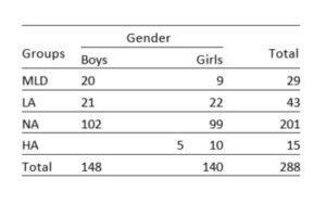
Researchers of mathematics learning difficulties (MLD) commonly use cutoff scores to determine which participants have MLD. These cutoff scores vary between -2 ss and -0.68 ss. Some researchers apply more restrictive cutoffs than others (e.g., performance below the 10th percentile or below the 35th percentile). The present study adopted the math achievement test to determine children with MLD based below the 10th percentile. The unit of analysis was third graders of an elementary school located in a low socioeconomic area. The study reached 288 students using math anxiety scale and math achievement test tools. The students were classified into four groups by their mathematics achievement test scores: math learning difficulties (0-10%), low achievers (11-25%), normal achievers (26-95%), and high achievers (96-100%).

Table 1. Distribution of participants by gender and groups

Data Collection Tools

Two copyrighted survey scales, consisting of 29 items were used to construct a survey questionnaire. The first scale is the Math Anxiety Scale developed by Mutlu & Söylemez for 3rd and 4th graders with a 3-factor structure of 13 items. The Cronbach’s Alpha coefficient is adopted by the study to evaluate the extent to which a measurement produces reliable results at different times. The Cronbach Alpha coefficient of the scale is .75 which confirms the reliability of and internal consistency of the study. The response set was designed in accordance with the three- point Likert scale with agree, neutral, and disagree. Of the 13 items in the scale, 5 were positive and 8 were negative. Positive items were rated as 3-2-1, while negative items were rated as 1-2-3. The highest score on the scale was 39 and the lowest on the scale was 13.

The second data collection tool adopted by this study is the math achievement test for third graders developed by Fidan (2013). It has 16 items designed in accordance with the national math curriculum. Correct responses were scored one point while wrong responses were scored zero point.

Data Analysis

The study mainly utilized five statistical analyses which are descriptive analysis, independent samples t-test, Pearson product-moment correlation analysis, linear regression and ANOVA. First, an independent samples t-test was performed to determine whether there was a significant difference between the levels of math anxiety by gender. Then, a Pearson product-moment correlation analysis was performed to determine the relationship between the math anxiety and mathematics achievement of the students. After that, a linear regression analysis was performed to predict the mathematics achievement of the participants based on their math anxiety. Finally, an ANOVA was performed to determine if there was a significant difference between the math anxiety of the groups determined in terms of mathematics achievement.

Results

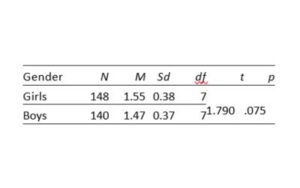
The findings of the math anxiety scores by gender of the study found no significant difference between the averages [t(286)= 1.790, p< .05]. This result shows that the math anxiety levels of girls and boys are close to each other. Since there is no difference between math anxiety scores by gender, the data in the study were combined.

Table 2. Comparison of anxiety scores by gender

There was a strong and negative correlation between math anxiety and mathematics achievement with the values of r= -0.597, n= 288, and p= .00. This result indicates that the highly math-anxious students and decreases in math anxiety were correlated with increases in rating of math achievement.

A simple linear regression was calculated to predict math achievement level based on the math anxiety. A significant regression equation was found (F(1,286)= 158.691, p< .000) with an R2 of .357. Participants’ predicted math achievement is equal to 20.153 + -6.611 when math anxiety is measured in unit. Math achievement decreased -6.611 for each unit of the math anxiety.

Figure below shows the relationship between the math anxiety of the children and their mathematics achievement on a group basis. Figure 1 provides us that there is a negative correlation between mathematical performance and math anxiety. The results depict that the HA group has the lowest math anxiety score, while the MLD group has the highest math anxiety.

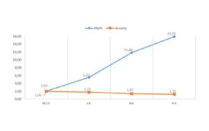
Table 3. Comparison of the mathematical anxiety scores of the groups

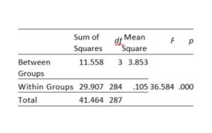
The table indicates that there is a statistically significant difference between groups as determined at the p<.05 level by one-way ANOVA (F(3,284)= 36.584, p= .000). Post hoc comparisons using the Tukey test indicated that the mean score for MLD group (M= 1.96, sd= 0.30) was significantly different than the NA group (M= 1.41, sd= 0.84) and HA group (M= 1.24, sd= 0.28). However, the MLD group (M= 1.96, sd= 0.30) did not significantly differ from the LA group (M= 1.76, sd= 0.27).

Discussion and Conclusion

Math anxiety is a problem that can adversely affect the academic success and employment prospects of children. Although the literature on math anxiety is largely focused on adults, recent studies have reported that some children begin to encounter math anxiety at the elementary school level. The findings of the study depict that the correlation level of math anxiety and math achievement is -.597 among students. In a meta-analysis study of Hembre and Ma, found that the level of relationship between mathematical success and math anxiety is -.34 and -.27, respectively. In a similar meta-analysis study performed in Turkey, the correlation coefficient was found to be -.44. The different occurrence of the coefficients is probably dependent on the scales used and the sample variety.

The participants of the study were classified into four groups: math learning difficulties (0-10%), low success (11-25%), normal (26-95%), and high success (96-100%) by the mathematics achievement test scores. The study compared the math anxiety scores of the groups and found no significant difference between the mean scores of the math anxiety of the lower two groups (mean of MLD math anxiety, .196; mean of LA math anxiety .177) as it was between the upper two groups (mean of NA math anxiety, .142; mean of HA math anxiety .125). This indicates that the math anxiety level of the students with learning difficulties in math does not differ from the low math students. However, a significant difference was found between the mean scores of math anxiety of the low successful and the normal group.

It may be better for some students to maintain moderate levels of math anxiety to make their learning and testing materials moderately challenging, but it can be clearly said that high math anxiety has detrimental effects on the mathematical performance of the individuals. Especially for students with learning difficulties in math, the high level of math anxiety will lead to destructive effects in many dimensions, primarily a lack of working memory.

Many of the techniques employed to reduce or eliminate the link between math anxiety and poor math performance involve addressing the anxiety rather than training math itself. Some methods for reducing math anxiety can be used in teaching mathematics. For instance, effective instruction for struggling mathematics learners includes instructional explicitness, a strong conceptual basis, cumulative review and practice, and motivators to help maintain student interest and engagement.

For more insights like this, visit our website at www.international-maths-challenge.com.

Credit for the article given to Yılmaz Mutlu