Category: mathematics

It could be argued that the square is the ‘nicest’ rhombus, but the rhombus with angles of 60 and 120 degrees seems nicer still. One of the nice things about the 60/120 rhomb are the plane tilings that can be constructed from it. One of these tilings is the ‘tumbling blocks’ tiling shown at the top of the post, in which at some points you see ‘cubes’ (around the degree 3 vertices), while at others you see ‘flowers’ (around the degree 6 vertices). Because of the two different types of vertices, this is known as a quasi-regular rhombic tiling. (Another tiling that uses the 60/120 rhomb is this one.)

If you want to build a polyhedron that resembles the tumbling block tiling, one method is to reduce the number of petals in your flowers to 5, and then stretch your 60/120 rhombs until they are have angles of 63.435 and 116.565 degrees. Thirty of these rhombs arranged around vertices of degree 3 and 5 produces a quasi-regular polygon known as the rhombic triacontahedron.

The image above is of a model that was built using rhombic units printed onto card stock.

Despite the apparent ugliness of the 63.435 and 116.565 degree angle-measurements, our nice 60/120 rhomb has been, arguably, stretched into an even nicer one – a ‘golden rhombus,’ so called because the ratio of the diagonals is equal to the golden ratio.

The dual of the rhombic triacontahedron is the archemedian polyhedron known as the icosidodecahedron.

For more such insights, log into www.international-maths-challenge.com.

*Credit for article given to dan.mackinnon*

The objects pictured above are interesting structures – they are derived from the prime factorization of a given number n. They can be described in a number of ways – for example, as directed graphs. Because they are nicely structured, they actually form something more special – a lattice. Accordingly, these structures are called factor lattices.
It’s easy to start drawing these by hand following the instructions below.

1. The first node is 1
2. Draw arrows out of this node for each of the prime factors of n.
3. The arrows that you just drew should connect to nodes labled with the prime factors of n.

Now, for each of the new nodes that you drew do the following:

4. Start from a node x that is not equal to n.
5. Draw arrows out of this node for each of the prime factors of n/x.
6. The arrows that you just drew (one for each p = n/x) should connect to nodes labled with the numbers p*x.

7. Now repeat 4,5, and 6 for each new node that you have drawn that is not equal to n.

This process is recursive, and ends when you have the complete lattice. The process is well suited for implementation as a computer program – the images above were created using SAGE using output from a Java program based on the algorithm above.

Manually trying out the steps out for a number like n = 24 goes something like this: First write out the prime factorization of 24, 24=(2*2*2)*3 = (2^3)*3. Starting with 1, draw arrows out to 2 and 3. Now looking at each node and following the algorithm, from the 2 you will get arrows out to 4 and 6. From the 3 you will get an arrow out to 6 as well. From 4 you will get arrows out to 8 or 12. From 6 you will get an arrow out to 12 as well. From 8 and from 12 you get arrows out to 24, and you are done.

In general, the algorithm produces a lattice that can be described as follows. Each node is a factor of the given number n. Two nodes are connected by an edge if their prime factorization differs by a single prime number. In other words, if a and b are nodes, and p = b/a, then there is an arrow p:a–>b.

It’s a good exercise to make the connections between the lattice structure and the prime factorization of a number n.

1. What does the factor lattice of a prime number look like?
2. If a number is just a power of a prime, what does its lattice look like?
3. If you know the factorization, can you find the number of nodes without drawing the lattice.

The answer to the last question (3) can be expressed as:

For example, if n = 24= 2^3*3, then the number of nodes will be (3+1)(1+1) = 8

That these structures can be thought of as “lattices”comes from the fact that you can think of the arrows as an ordering of the nodes, ab. The number 1 is always the least node in the factor lattice for n, while n itself is the greatest node. The property that actually makes these structures a “lattice” is that for any two nodes there is always a lower-bound for any pair of nodes in the lattice, and always an upper-bound for the pair (these are often referred to as meets and joins).

The Wolfram Demonstrations Project has a nice factor lattice demo that will draw factor lattices for a large number of integers for you. There is also a good Wikipedia entry for lattices in general.

For more such insights, log into www.international-maths-challenge.com.

*Credit for article given to dan.mackinnon*

For everyone whose relationship with mathematics is distant or broken, Jo Boaler, a professor at Stanford Graduate School of Education (GSE), has ideas for repairing it. She particularly wants young people to feel comfortable with numbers from the start—to approach the subject with playfulness and curiosity, not anxiety or dread.

“Most people have only ever experienced what WEcall narrow mathematics—a set of procedures they need to follow, at speed,” Boaler says. “Mathematics should be flexible, conceptual, a place where we play with ideas and make connections. If we open it up and invite more creativity, more diverse thinking, we can completely transform the experience.”

Boaler, the Nomellini and Olivier Professor of Education at the GSE, is the co-founder and faculty director of Youcubed, a Stanford research center that provides resources for math learning that has reached more than 230 million students in over 140 countries. In 2013 Boaler, a former high school math teacher, produced How to Learn Math, the first massive open online course (MOOC) on mathematics education. She leads workshops and leadership summits for teachers and administrators, and her online courses have been taken by over a million users.

In her new book, “Math-ish: Finding Creativity, Diversity, and Meaning in Mathematics,” Boaler argues for a broad, inclusive approach to math education, offering strategies and activities for learners at any age. We spoke with her about why creativity is an important part of mathematics, the impact of representing numbers visually and physically, and how what she calls “ishing” a math problem can help students make better sense of the answer.

What do you mean by ‘math-ish’ thinking?

It’s a way of thinking about numbers in the real world, which are usually imprecise estimates. If someone asks how old you are, how warm it is outside, how long it takes to drive to the airport—these are generally answered with what WEcall “ish” numbers, and that’s very different from the way we use and learn numbers in school.

In the book WEshare an example of a multiple-choice question from a nationwide exam where students are asked to estimate the sum of two fractions: 12/13 + 7/8. They’re given four choices for the closest answer: 1, 2, 19, or 21. Each of the fractions in the question is very close to 1, so the answer would be 2—but the most common answer 13-year-olds gave was 19. The second most common was 21.

I’m not surprised, because when students learn fractions, they often don’t learn to think conceptually or to consider the relationship between the numerator or denominator. They learn rules about creating common denominators and adding or subtracting the numerators, without making sense of the fraction as a whole. But stepping back and judging whether a calculation is reasonable might be the most valuable mathematical skill a person can develop.

But don’t you also risk sending the message that mathematical precision isn’t important?

I’m not saying precision isn’t important. What I’m suggesting is that we ask students to estimate before they calculate, so when they come up with a precise answer, they’ll have a real sense for whether it makes sense. This also helps students learn how to move between big-picture and focused thinking, which are two different but equally important modes of reasoning.

Some people ask me, “Isn’t ‘ishing’ just estimating?” It is, but when we ask students to estimate, they often groan, thinking it’s yet another mathematical method. But when we ask them to “ish” a number, they’re more willing to offer their thinking.

Ishing helps students develop a sense for numbers and shapes. It can help soften the sharp edges in mathematics, making it easier for kids to jump in and engage. It can buffer students against the dangers of perfectionism, which we know can be a damaging mindset. WEthink we all need a little more ish in our lives.

You also argue that mathematics should be taught in more visual ways. What do you mean by that?

For most people, mathematics is an almost entirely symbolic, numerical experience. Any visuals are usually sterile images in a textbook, showing bisecting angles, or circles divided into slices. But the way we function in life is by developing models of things in our minds. Take a stapler: Knowing what it looks like, what it feels and sounds like, how to interact with it, how it changes things—all of that contributes to our understanding of how it works.

There’s an activity we do with middle-school students where we show them an image of a 4 x 4 x 4 cm cube made up of smaller 1 cm cubes, like a Rubik’s Cube. The larger cube is dipped into a can of blue paint, and we ask the students, if they could take apart the little cubes, how many sides would be painted blue? Sometimes we give the students sugar cubes and have them physically build a larger 4 x 4 x 4 cube. This is an activity that leads into algebraic thinking.

Some years back we were interviewing students a year after they’d done that activity in our summer camp and asked what had stayed with them. One student said, “I’m in geometry class now, and We still remember that sugar cube, what it looked like and felt like.” His class had been asked to estimate the volume of their shoes, and he said he’d imagined his shoes filled with 1 cm sugar cubes in order to solve that question. He had built a mental model of a cube.

When we learn about cubes, most of us don’t get to see and manipulate them. When we learn about square roots, we don’t take squares and look at their diagonals. We just manipulate numbers.

WEwonder if people consider the physical representations more appropriate for younger kids.

That’s the thing—elementary school teachers are amazing at giving kids those experiences, but it dies out in middle school, and by high school it’s all symbolic. There’s a myth that there’s a hierarchy of sophistication where you start out with visual and physical representations and then build up to the symbolic. But so much of high-level mathematical work now is visual. Here in Silicon Valley, if you look at Tesla engineers, they’re drawing, they’re sketching, they’re building models, and nobody says that’s elementary mathematics.

There’s an example in the book where you’ve asked students how they would calculate 38 x 5 in their heads, and they come up with several different ways of arriving at the same answer. The creativity is fascinating, but wouldn’t it be easier to teach students one standard method?

That narrow, rigid version of mathematics where there’s only one right approach is what most students experience, and it’s a big part of why people have such math trauma. It keeps them from realizing the full range and power of mathematics. When you only have students blindly memorizing math facts, they’re not developing number sense.

They don’t learn how to use numbers flexibly in different situations. It also makes students who think differently believe there’s something wrong with them.

For more such insights, log into our website https://international-maths-challenge.com

Credit of the article given to Stanford University

John Sims has created a number of pi-related art works. One, the Pi Color Map, can be recreated effectively using TinkerPlots. The image above is one such Pi Color Map, using 2281 digits of pi.

Here are some instructions for creating a Pi Color Map in Tinkerplots.

1. Obtain a listing of the digits of pi – up to a reasonable number. You can get the digits from several sites, including the pi day site.

2. Paste your listing to a text document, and get them arranged into a single column. One strategy for doing this is and use the find/replace feature of a word-processor to replace each number with the number itself plus a line-break(e.g. in Word, replace 2 with 2^l, etc.).

3. If you’ve included the decimal point, remove it. For the first line of your document, provide a heading like pi_expansion. This will be your TinkerPlots attribute.

3. Import the text file into TinkerPlots using the File>Import menu.

4. Create a new attribute called digit whose formula is digit=concat(“”,pi_expansion). This creates a categorical data type that TinkerPlots won’t treat numerically. This is what you will use as your color key. Using the pi_expansion attribute gives a spectrum of color, rather than distinct colors for each number.

5. Create a new attribute called place, whose formula is place=caseIndex. This is what you will order your plot by.

6. Create a new plot, lock the color key on the digit attribute. Select the place attribute and press the Order By button.

7. Change your icon type to small squares, and stack the cases.

You can play with different options to get different effects for your color map.

One nice thing about doing this in TinkerPlots is that you can investigate the data further. The color map plot highlights the apparent randomness of the pi expansion, but you can also create other attributes and plots to investigate things like the running average of the digits, occurrences of consecutive digits, and the overall distribution of the digits (it should be uniform).

For more such insights, log into www.international-maths-challenge.com.

*Credit for article given to dan.mackinnon*

Today I’d like to share an idea. It’s a very simple idea. It’s not fancy and it’s certainly not new. In fact, I’m sure many of you have thought about it already. But if you haven’t—and even if you have!—I hope you’ll take a few minutes to enjoy it with me. Here’s the idea:

So simple! But we can get a lot of mileage out of it.

To start, I’ll be a little more precise: every matrix corresponds to a weighted bipartite graph. By “graph” I mean a collection of vertices (dots) and edges; by “bipartite” I mean that the dots come in two different types/colors; by “weighted” I mean each edge is labeled with a number.

The graph above corresponds to a 3×23×2 matrix MM. You’ll notice I’ve drawn three greengreen dots—one for each row of MM—and two pinkpink dots—one for each column of MM. I’ve also drawn an edge between a green dot and a pink dot if the corresponding entry in MM is non-zero.

For example, there’s an edge between the second green dot and the first pink dot because M21=4M21=4, the entry in the second row, first column of MM, is not zero. Moreover, I’ve labeled that edge by that non-zero number. On the other hand, there is no edge between the first green dot and the second pink dot because M12M12, the entry in the first row, second column of the matrix, is zero.

Allow me to describe the general set-up a little more explicitly.

Any matrix MM is an array of n×mn×m numbers. That’s old news, of course. But such an array can also be viewed as a function M:X×Y→RM:X×Y→R where X={x1,…,xn}X={x1,…,xn} is a set of nn elements and Y={y1,…,ym}Y={y1,…,ym} is a set of mm elements. Indeed, if I want to describe the matrix MM to you, then I need to tell you what each of its ijijth entries are. In other words, for each pair of indices (i,j)(i,j), I need to give you a real number MijMij. But that’s precisely what a function does! A function M:X×Y→RM:X×Y→R associates for every pair (xi,yj)(xi,yj) (if you like, just drop the letters and think of this as (i,j)(i,j)) a real number M(xi,yj)M(xi,yj). So simply write MijMij for M(xi,yj)M(xi,yj).

Et voila. A matrix is a function.

For more such insights, log into www.international-maths-challenge.com.

*Credit for article given to Tai-Danae Bradley*

It’s a bit more complicated than this

Forget your times tables – mathematicians have found a new, faster way to multiply two numbers together. The method, which works only for whole numbers, is a landmark result in computer science. “This is big news,” says Joshua Cooper at the University of South Carolina.

To understand the new technique, which was devised by David Harvey at the University of New South Wales, Australia, and Joris van der Hoeven at the Ecole Polytechnique near Paris, France, it helps to think back to the longhand multiplication you learned at school.

We write down two numbers, one on top of the other, and then painstakingly multiply each digit of one by each digit of the other, before adding all the results together. “This is an ancient algorithm,” says Cooper.

If your two numbers each have n digits, this way of multiplying will require roughly n² individual calculations. “The question is, can you do better?” says Cooper.

Lots of logs

Starting in the 1960s, mathematicians began to prove that they could. First Anatoly Karatsuba found an algorithm that could turn out an answer in no more than n^1.58 steps, and in 1971, Arnold Schönhage and Volker Strassen found a way to peg the number of steps to the complicated expression n*(log(n))*log(log(n)) – here “log” is short for logarithm.

These advances had a major impact on computing. Whereas a computer using the longhand multiplication method would take about six months to multiply two billion-digit numbers together, says Harvey, the Schönhage-Strassen algorithm can do it in 26 seconds.

The landmark 1971 paper also suggested a possible improvement, a tantalising prediction that multiplication might one day be possible in no more than n*log(n) steps. Now Harvey and van der Hoeven appear to have proved this is the case. “It finally appears to be possible,” says Cooper. “It passes the smell test.”

“If the result is correct, it’s a major achievement in computational complexity theory,” says Fredrik Johansson at INRIA, the French research institute for digital sciences, in Bordeaux. “The new ideas in this work are likely to inspire further research and could lead to practical improvements down the road.”

Cooper also praises the originality of the research, although stresses the complexity of the mathematics involved. “You think, jeez, I’m just multiplying two integers, how complicated can it get?” says Cooper. “But boy, it gets complicated.”

So, will this make calculating your tax returns any easier? “For human beings working with pencil and paper, absolutely not,” says Harvey. Indeed, their version of the proof only works for numbers with more than 10 to the power of 200 trillion trillion trillion digits. “The word ‘astronomical’ falls comically short in trying to describe this number,” says Harvey.

While future improvements to the algorithm may extend the proof to more humdrum numbers only a few trillion digits long, Cooper thinks its real value lies elsewhere. From a theoretical perspective, he says, this work allows programmers to provide a definitive guarantee of how long a certain algorithm will take. “We are optimistic that our new paper will allow us to achieve further practical speed-ups,” says van der Hoeven.

Harvey thinks this may well be the end of the story, with no future algorithm capable of beating n*log(n). “I would be extremely surprised if this turned out to be wrong,” he says, “but stranger things have happened.”

For more such insights, log into www.international-maths-challenge.com.

*Credit for article given to Gilead Amit*

A surprisingly interesting structure is the extended multiplication table, shown above for the numbers seven to ten. The algorithm for drawing these is straight forward – for an n-extended table, start out as if you were writing a “regular” multiplication table, but extend each row so that it gets as close to, without exceeding, n. Another way to think about it is to write out rows of “skip counting up to n” by i for integers i from 1 to n.

This is called an extended multiplication table since it contains a “traditional” multiplication table inside it. The 12-extended table below contains a traditional 3×3 multiplication table.

It turns out that 1 appears in an extended table once, and prime numbers appear exactly twice (once in the first column, and once in the first row). In general, for a natural number n, how many times does n appear in the n-extended table?

Before looking at that question, you might want to think about finding easier ways to draw the tables. Drawing out these tables by hand can be tedious – a simple program or spreadsheet might be easier. You can use Fathom, for example, to create the table data and draw it in the collections display. Create a slider m and the attributes listed in the table below (click on the image to see a larger version).

Modify the collection display attributes to draw the tables in the collection box. By adding lots of cases and using the slider m to filter out the ones you don’t need, you can vary the size of the table easily.

“how many times does n appear in the n-extended table?”

# of occurrances of n in the n-extended table = # of nodes in the factor lattice Fn

You can also recast both of these questions (how many occurances of n in the n-extended table, and how many nodesin the Fn factor lattice) as a combinatorial “balls in urns” problem.

Consider a set of colored balls where there are m different colours, where there are ki balls of color i, where i ranges from 1 to m. This would give a total number of balls equal to k1+k2+…+km. Suppose you were to distribute these balls in two urns. How many different distributions would there be? Using some counting techniques, you will find that the answer is (k1+1)*(k2+1)*…*(km+1).

How is this connected to the other problems? Consider the prime factorization of the number. For each prime, choose a colour, and for each occurance of the prime in the factorization, add a new ball of that color. For example for 12 = 3*3*2, choose two colours – say blue=3 and red=2. Since 3 occurs twice and 2 occurs once, there should be two blue balls and one red ball. Now consider distributing these balls in two urns. It turns out that you get (2+1)*(1+1) = 6 possibilities. This is the same number of times 12 occurs in the 12-extended table, and the same number of nodes in the 12-factor lattice. The image below shows the 12-extended table, the 12-factor lattice, and the “ball and urn problem” for the numer 12.

For a number n with the prime factorization:

The answer to all three questions is given by:

For more such insights, log into www.international-maths-challenge.com.

*Credit for article given to dan.mackinnon*

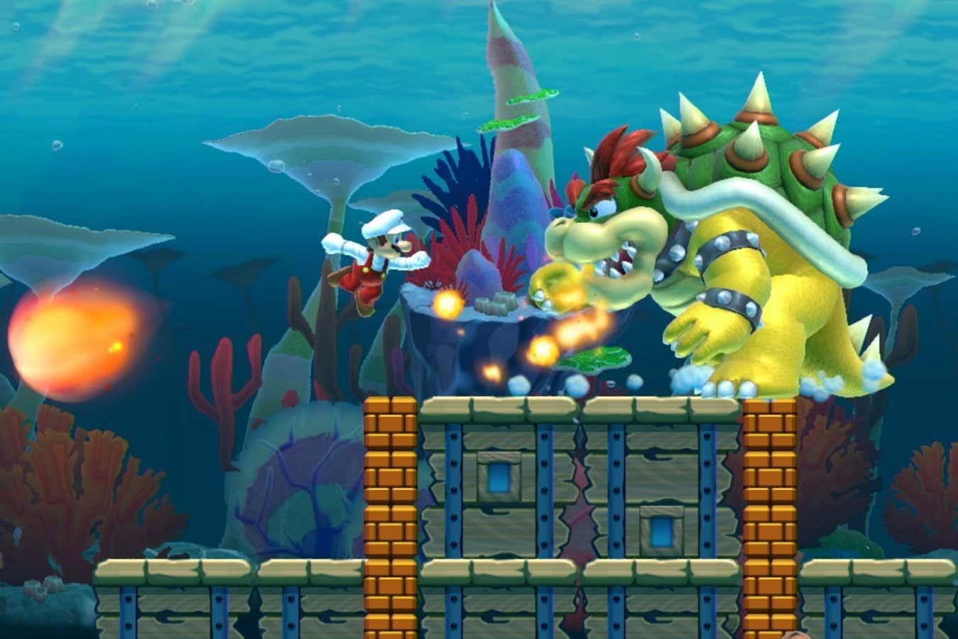
Using the tools of computational complexity, researchers have discovered it is impossible to figure out whether certain Super Mario Bros levels can be beaten without playing them, even if you use the world’s most powerful supercomputer.

Figuring out whether certain levels in the Super Mario Bros series of video games can be completed before you play them is mathematically impossible, even if you had several years and the world’s most powerful supercomputer to hand, researchers have found.

“We don’t know how to prove that a game is fun, we don’t know what that means mathematically, but we can prove that it’s hard and that maybe gives some insight into why it’s fun,” says Erik Demaine at the Massachusetts Institute of Technology. “I like to think of hard as a proxy for fun.”

To prove this, Demaine and his colleagues use tools from the field of computational complexity – the study of how difficult and time-consuming various problems are to solve algorithmically. They have previously proven that figuring out whether it is possible to complete certain levels in Mario games is a task that belongs to a group of problems known as NP-hard, where the complexity grows exponentially. This category is extremely difficult to compute for all but the smallest problems.

Now, Demaine and his team have gone one step further by showing that, for certain levels in Super Mario games, answering this question is not only hard, but impossible. This is the case for several titles in the series, including New Super Mario Bros and Super Mario Maker. “You can’t get any harder than this,” he says. “Can you get to the finish? There is no algorithm that can answer that question in a finite amount of time.”

While it may seem counterintuitive, problems in this undecidable category, known as RE-complete, simply cannot be solved by a computer, no matter how powerful, no matter how long you let it work.

Demaine concedes that a small amount of trickery was needed to make Mario levels fit this category. Firstly, the research looks at custom-made levels that allowed the team to place hundreds or thousands of enemies on a single spot. To do this they had to remove the limits placed by the game publishers on the number of enemies that can be present in a level.

They were then able to use the placement of enemies within the level to create an abstract mathematical tool called a counter machine, essentially creating a functional computer within the game.

That trick allowed the team to invoke another conundrum known as the halting problem, which says that, in general, there is no way to determine if a given computer program will ever terminate, or simply run forever, other than running it and seeing what happens.

These layers of mathematical concepts finally allowed the team to prove that no analysis of the game level can say for sure whether or not it can ever be completed. “The idea is that you’ll be able to solve this Mario level only if this particular computation will terminate, and we know that there’s no way to determine that, and so there’s no way to determine whether you can solve the level,” says Demaine.

For more such insights, log into www.international-maths-challenge.com.

*Credit for article given to Matthew Sparkes*

These are painful times for those hoping to see an international consensus and substantive action on global warming.

In the US, Republican presidential front-runner Mitt Romney said in June 2011: “The world is getting warmer” and “humans have contributed” but in October 2011 he backtracked to: “My view is that we don’t know what’s causing climate change on this planet.”

His Republican challenger Rick Santorum added: “We have learned to be sceptical of ‘scientific’ claims, particularly those at war with our common sense” and Rick Perry, who suspended his campaign to become the Republican presidential candidate last month, stated flatly: “It’s all one contrived phony mess that is falling apart under its own weight.”

Meanwhile, the scientific consensus has moved in the opposite direction. In a study published in October 2011, 97% of climate scientists surveyed agreed global temperatures have risen over the past 100 years. Only 5% disagreed that human activity is a significant cause of global warming.

The study concluded in the following way: “We found disagreement over the future effects of climate change, but not over the existence of anthropogenic global warming.

“Indeed, it is possible that the growing public perception of scientific disagreement over the existence of anthropocentric warming, which was stimulated by press accounts of [the UK’s] ”Climategate“ is actually a misperception of the normal range of disagreements that may persist within a broad scientific consensus.”

More progress has been made in Europe, where the EU has established targets to reduce emissions by 20% (from 1990 levels) by 2020. The UK, which has been beset by similar denial movements, was nonetheless able to establish, as a legally binding target, an 80% reduction by 2050 and is a world leader on abatement.

In Australia, any prospect for consensus was lost when Tony Abbott used opposition to the Labor government’s proposed carbon market to replace Malcolm Turnbull as leader of the Federal Opposition in late 2009.

It used to be possible to hear right-wing politicians in Australia or the USA echo the Democratic congressman Henry Waxman who said last year:

“If my doctor told me I had cancer, I wouldn’t scour the country to find someone to tell me that I don’t need to worry about it.”

But such rationality has largely left the debate in both the US and Oz. In Australia, a reformulated carbon tax policy was enacted in November only after a highly partisan debate.

In Canada, the debate is a tad more balanced. The centre-right Liberal government in British Columbia passed the first carbon tax in North America in 2008, but the governing Federal Conservative party now offers a reliable “anti-Kyoto” partnership with Washington.

Overviews of the evidence for global warming, together with responses to common questions, are available from various sources, including:

• Seven Answers to Climate Contrarian Nonsense, in Scientific American
• Climate change: A Guide for the Perplexed, in New Scientist
• Cooling the Warming Debate: Major New Analysis Confirms That Global Warming Is Real, in Science Daily
• Remind me again: how does climate change work? on The Conversation

It should be acknowledged in these analyses that all projections are based on mathematical models with a significant level of uncertainty regarding highly complex and only partially understood systems.

As 2011 Australian Nobel-Prize-winner Brian Schmidt explained while addressing a National Forum on Mathematical Education:

“Climate models have uncertainty and the earth has natural variation … which not only varies year to year, but correlates decade to decade and even century to century. It is really hard to design a figure that shows this in a fair way — our brain cannot deal with the correlations easily.

“But we do have mathematical ways of dealing with this problem. The Australian academy reports currently indicate that the models with the effects of CO₂ are with 90% statistical certainty better at explaining the data than those without.

“Most of us who work with uncertainty know that 90% statistical uncertainty cannot be easily shown within a figure — it is too hard to see …”

“ … Since predicting the exact effects of climate change is not yet possible, we have to live with uncertainty and take the consensus view that warming can cover a wide range of possibilities, and that the view might change as we learn more.”

But uncertainty is no excuse for inaction. The proposed counter-measures (e.g. infrastructure renewal and modernisation, large-scale solar and wind power, better soil remediation and water management, not to mention carbon taxation) are affordable and most can be justified on their own merits, while the worst-case scenario — do nothing while the oceans rise and the climate changes wildly — is unthinkable.

Some in the first world protest that any green energy efforts are dwarfed by expanding energy consumption in China and elsewhere. Sure, China’s future energy needs are prodigious, but China also now leads the world in green energy investment.

By blaiming others and focusing the debate on the level of human responsibility for warming and about the accuracy of predictions, the deniers have managed to derail long-term action in favour of short-term economic policies.

Who in the scientific community is promoting the denial of global warming? As it turns out, the leading figures in this movement have ties to conservative research institutes funded mostly by large corporations, and have a history of opposing the scientific consensus on issues such as tobacco and acid rain.

What’s more, those who lead the global warming denial movement – along with creationists, intelligent design writers and the “mathematicians” who flood our email inboxes with claims that pi is rational or other similar nonsense – are operating well outside the established boundaries of peer-reviewed science.

Austrian-born American physicist Fred Singer, arguably the leading figure of the denial movement, has only six peer-reviewed publications in the climate science field, and none since 1997.

After all, when issues such as these are “debated” in any setting other than a peer-reviewed journal or conference, one must ask: “If the author really has a solid argument, why isn’t he or she back in the office furiously writing up this material for submission to a leading journal, thereby assuring worldwide fame and glory, not to mention influence?”

In most cases, those who attempt to grab public attention through other means are themselves aware they are short-circuiting the normal process, and that they do not yet have the sort of solid data and airtight arguments that could withstand the withering scrutiny of scientific peer review.

When they press their views in public to a populace that does not understand how the scientific enterprise operates, they are being disingenuous.

With regards to claims scientists are engaged in a “conspiracy” to hide the “truth” on an issue such as global warming or evolution, one should ask how a secret “conspiracy” could be maintained in a worldwide, multicultural community of hundreds of thousands of competitive researchers.

As Benjamin Franklin wrote in his Poor Richard’s Almanac: “Three can keep a secret, provided two of them are dead.” Or as one of your present authors quipped, tongue-in-cheek, in response to a state legislator who was skeptical of evolution: “You have no idea how humiliating this is to me — there is a secret conspiracy among leading scientists, but no-one deemed me important enough to be included!”

There’s another way to think about such claims: we have tens-of-thousands of senior scientists in their late-fifties or early-sixties who have seen their retirement savings decimated by the recent stock market plunge. These are scientists who now wonder if the day will ever come when they are financially well-off-enough to do their research without the constant stress and distraction of applying for grants (the majority of which are never funded).

All one of these scientists has to do to garner both worldwide fame and considerable fortune (through book contracts, the lecture circuit and TV deals) is to call a news conference and expose “the truth”. So why isn’t this happening?

The system of peer-reviewed journals and conferences sponsored by major professional societies is the only proper forum for the presentation and debate of new ideas, in any field of science or mathematics.

It has been stunningly successful: errors have been uncovered, fraud has been rooted out and bogus scientific claims (such as the 1903 N-ray claim, the 1989 cold fusion claim, and the more-recent assertion of an autism-vaccination link) have been debunked.

This all occurs with a level of reliability and at a speed that is hard to imagine in other human endeavours. Those who attempt to short-circuit this system are doing potentially irreparable harm to the integrity of the system.

They may enrich themselves or their friends, but they are doing grievous damage to society at large.

For more such insights, log into our website https://international-maths-challenge.com

Credit of the article given to Jonathan Borwein (Jon), University of Newcastle and David H. Bailey, University of California, Davis

Our laws of nature are written in the language of mathematics. But maths itself is only as dependable as the axioms it is built on, and we have to assume those axioms are true.

You might think that mathematics is the most trustworthy thing humans have ever come up with. It is the basis of scientific rigour and the bedrock of much of our other knowledge too. And you might be right. But be careful: maths isn’t all it seems. “The trustworthiness of mathematics is limited,” says Penelope Maddy, a philosopher of mathematics at the University of California, Irvine.

Maddy is no conspiracy theorist. All mathematicians know her statement to be true because their subject is built on “axioms” – and try as they might, they can never prove these axioms to be true.

An axiom is essentially an assumption based on observations of how things are. Scientists observe a phenomenon, formalise it and write down a law of nature. In a similar way, mathematicians use their observations to create an axiom. One example is the observation that there always seems to be a unique straight line that can be drawn between two points. Assume this to be universally true and you can build up the rules of Euclidean geometry. Another is that 1 + 2 is the same as 2 + 1, an assumption that allows us to do arithmetic. “The fact that maths is built on unprovable axioms is not that surprising,” says mathematician Vera Fischer at the University of Vienna in Austria.

These axioms might seem self-evident, but maths goes a lot further than arithmetic. Mathematicians aim to uncover things like the properties of numbers, the ways in which they are all related to one another and how they can be used to model the real world. These more complex tasks are still worked out through theorems and proofs built on axioms, but the relevant axioms might have to change. Lines between points have different properties on curved surfaces than flat ones, for example, which means the underlying axioms have to be different in different geometries. We always have to be careful that our axioms are reliable and reflect the world we are trying to model with our maths.

Set theory

The gold standard for mathematical reliability is set theory, which describes the properties of collections of things, including numbers themselves. Beginning in the early 1900s, mathematicians developed a set of underpinning axioms for set theory known as ZFC (for “Zermelo-Fraenkel”, from two of its initiators, Ernst Zermelo and Abraham Fraenkel, plus something called the “axiom of choice”).

ZFC is a powerful foundation. “If it could be guaranteed that ZFC is consistent, all uncertainty about mathematics could be dispelled,” says Maddy. But, brutally, that is impossible. “Alas, it soon became clear that the consistency of those axioms could be proved only by assuming even stronger axioms,” she says, “which obviously defeats the purpose.”

Maddy is untroubled by the limits: “Set theorists have been proving theorems from ZFC for 100 years with no hint of a contradiction.” It has been hugely productive, she says, allowing mathematicians to create no end of interesting results, and they have even been able to develop mathematically precise measures of just how much trust we can put in theories derived from ZFC.

In the end, then, mathematicians might be providing the bedrock on which much scientific knowledge is built, but they can’t offer cast-iron guarantees that it won’t ever shift or change. In general, they don’t worry about it: they shrug their shoulders and turn up to work like everybody else. “The aim of obtaining a perfect axiomatic system is exactly as feasible as the aim of obtaining a perfect understanding of our physical universe,” says Fischer.

At least mathematicians are fully aware of the futility of seeking perfection, thanks to the “incompleteness” theorems laid out by Kurt Gödel in the 1930s. These show that, in any domain of mathematics, a useful theory will generate statements about this domain that can’t be proved true or false. A limit to reliable knowledge is therefore inescapable. “This is a fact of life mathematicians have learned to live with,” says David Aspero at the University of East Anglia, UK.

All in all, maths is in pretty good shape despite this – and nobody is too bothered. “Go to any mathematics department and talk to anyone who’s not a logician, and they’ll say, ‘Oh, the axioms are just there’. That’s it. And that’s how it should be. It’s a very healthy approach,” says Fischer. In fact, the limits are in some ways what makes it fun, she says. “The possibility of development, of getting better, is exactly what makes mathematics an absolutely fascinating subject.”

HOW BIG IS INFINITY?

Infinity is infinitely big, right? Sadly, it isn’t that simple. We have long known that there are different sizes of infinity. In the 19th century, mathematician Georg Cantor showed that there are two types of infinity. The “natural numbers” (1, 2, 3 and so on forever) are a countable infinity. But between each natural number, there is a continuum of “real numbers” (such as 1.234567… with digits that go on forever). Real number infinities turn out not to be countable. And so, overall, Cantor concluded that there are two types of infinity, each of a different size.

In the everyday world, we never encounter anything infinite. We have to content ourselves with saying that the infinite “goes on forever” without truly grasping conceptually what that means. This matters, of course, because infinities crop up all the time in physics equations, most notably in those that describe the big bang and black holes. You might have expected mathematicians to have a better grasp of this concept, then – but it remains tricky.

This is especially true when you consider that Cantor suggested there might be another size of infinity nestled between the two he identified, an idea known as the continuum hypothesis. Traditionally, mathematicians thought that it would be impossible to decide whether this was true, but work on the foundations of mathematics has recently shown that there may be hope of finding out either way after all.

For more such insights, log into www.international-maths-challenge.com.

*Credit for article given to Michael Brooks*