This post is the third example in an ongoing list of various sequences of functions which converge to different things in different ways.
Example 3
A sequence of continuous functions {fn:R→[0,∞)}{fn:R→[0,∞)} which converges to 0 in the L1L1 norm, but does not converge to 0 uniformly.
There are four criteria we want our functions to satisfy:
- First off is the uniform convergence. Observe that “{fn}{fn} does not converge to 0 uniformly” can mean one of three things:
- converges to 0 pointwise only
- converges to something other than 0 (pointwise or uniformly)
- does not converge at all
So it’s up to you to decide which one feels more comfortable to work with. Here we’ll choose the second option.
- Next, “{fn}{fn} converges to 0 in the L1L1 norm” means that we want to choose our sequence so that the area under the curve of the fnfn gets smaller and smaller as n→∞n→∞.
- Further, we also want the fnfn to be positive (the image of each fnfn must be [0,∞)[0,∞)) (notice this allows us to remove the abosolute value sign in the L1L1 norm: ∫|fn|⇒∫fn∫|fn|⇒∫fn)
- Lastly, the functions must be continuous.
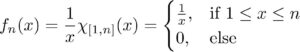
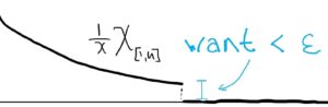
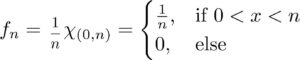
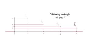
A slick* but very simple solution is a sequence of triangles of decreasing area with height 1!
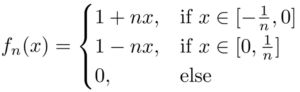
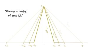
This works because: At x=0x=0, fn(x)=1fn(x)=1 for all nn, so there’s no way it can converge to zero (much less uniformly). In fact we have fn→ffn→f pointwise wheref(x)={1,if x=00otherwise.f(x)={1,if x=00otherwise.The area of each triangle is 1n1n which clearly goes to zero for nn large. Also, it’s clear to see visually that the area is getting smaller. This guarantees fn→0fn→0 in the L1L1 norm. Further, each fnfn is positive since we’ve defined it to equal zero as soon as the edges of the triangle reach the xx-axis. And lastly we have piecewise continuity.
The details: Let ϵ>0ϵ>0 and x∈Rx∈R. If x=0x=0, then fn(x)=1fn(x)=1 for all n and so fn→1fn→1. Otherwise x>0x>0 or x<0x<0 If x>0x>0 and x>1x>1, then fn(x)=0fn(x)=0 for all nn. Otherwise if x∈(0,1]x∈(0,1] choose N>1xN>1x. Then whenever n>Nn>N we have fn(x)=1−nx<1−1xx=0<ϵ.fn(x)=1−nx<1−1xx=0<ϵ. The case when x<0x<0 follows a similar argument.
Lastly fn→0fn→0 in the L1L1 norm since, as we mentioned, the areas are decreasing to 0. Explicitly: ∫R|fn|=∫0−1n1+nx+∫1n01−nx=2n→0.∫R|fn|=∫−1n01+nx+∫01n1−nx=2n→0.
*I can brag because this particular example came from a friend. My own attempt at a solution was not nearly as intuitive.
Constructing the Tensor Product of Modules
The Basic Idea

Today we talk tensor products. Specifically this post covers the construction of the tensor product between two modules over a ring. But before jumping in, I think now’s a good time to ask, “What are tensor products good for?” Here’s a simple example where such a question might arise:
Suppose you have a vector space VV over a field FF. For concreteness, let’s consider the case when VV is the set of all 2×22×2 matrices with entries in RR and let F=RF=R. In this case we know what “FF-scalar multiplication” means: if M∈VM∈V is a matrix and c∈Rc∈R, then the new matrix cMcM makes perfect sense. But what if we want to multiply MM by complex scalars too? How can we make sense of something like (3+4i)M(3+4i)M? That’s precisely what the tensor product is for! We need to create a set of elements of the form(complex number) “times” (matrix)(complex number) “times” (matrix)so that the mathematics still makes sense. With a little massaging, this set will turn out to be C⊗RVC⊗RV.
So in general, if FF is an arbitrary field and VV an FF-vector space, the tensor product answers the question “How can I define scalar multiplication by some larger field which contains FF?” And of course this holds if we replace the word “field” by “ring” and consider the same scenario with modules.
Now this isn’t the only thing tensor products are good for (far from it!), but I think it’s the most intuitive one since it is readily seen from the definition (which is given below).
So with this motivation in mind, let’s go!
From English to Math
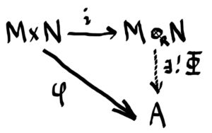
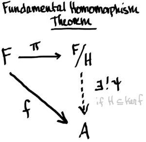
Let RR be a ring with 1 and let MM be a right RR-module and NN a left RR-module and suppose AA is any abelian group. Our goal is to create an abelian group M⊗RNM⊗RN, called the tensor product of MM and NN, such that if there is an RR-balanced map i:M×N→M⊗RNi:M×N→M⊗RN and any RR-balanced map φ:M×N→Aφ:M×N→A, then there is a unique abelian group homomorphism Φ:M⊗RN→AΦ:M⊗RN→A such that φ=Φ∘iφ=Φ∘i, i.e. so the diagram below commutes.
Notice that the statement above has the same flavor as the universal mapping property of free groups!
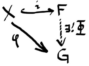
Definition: Let XX be a set. A group FF is said to be a free group on XX if there is a function i:X→Fi:X→F such that for any group GG and any set map φ:X→Gφ:X→G, there exists a unique group homomorphism Φ:F→GΦ:F→G such that the following diagram commutes: (i.e. φ=Φ∘iφ=Φ∘i)
set map, so in particular we just want our’s to be RR-balanced:
: Let RR be a ring with 1. Let MM be a right RR-module, NN a left RR-module, and AA an abelian group. A map φ:M×N→Rφ:M×N→R is called RR-balanced if for all m,m1,m2∈Mm,m1,m2∈M, all n,n1,n2∈Nn,n1,n2∈N and all r∈Rr∈R,
φ(m1+m2,n)=φ(m1,n)+φ(m2,n)φ(m1+m2,n)=φ(m1,n)+φ(m2,n)φ(m,n1+n2)=φ(m,n1)+φ(m,n2)φ(m,n1+n2)=φ(m,n1)+φ(m,n2)φ(mr,n)=φ(m,rn)φ(mr,n)=φ(m,rn)
By “replacing” F by a certain quotient group F/HF/H! (We’ll define HH precisely below.)
These observations give us a road map to construct the tensor product. And so we begin:
Step 1
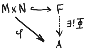
Let FF be a free abelian group generated by M×NM×N and let AA be an abelian group. Then by definition (of free groups), if φ:M×N→Aφ:M×N→A is any set map, and M×N↪FM×N↪F by inclusion, then there is a unique abelian group homomorphism Φ:F→AΦ:F→A so that the following diagram commutes.
Step 2
that the inclusion map M×N↪FM×N↪F is not RR-balanced! To fix this, we must “modify” the target space FF by replacing it with the quotient F/HF/H where H≤FH≤F is the subgroup of FF generated by elements of the form
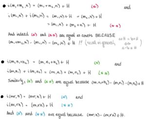
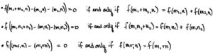
(m1+m2,n)−(m1,n)−(m2,n)(m1+m2,n)−(m1,n)−(m2,n)
- (m,n1+n2)−(m,n1)−(m,n2)(m,n1+n2)−(m,n1)−(m,n2)
- (mr,n)−(m,rn)(mr,n)−(m,rn)
where m1,m2,m∈Mm1,m2,m∈M, n1,n2,n∈Nn1,n2,n∈N and r∈Rr∈R. Why elements of this form? Because if we define the map i:M×N→F/Hi:M×N→F/H byi(m,n)=(m,n)+H,i(m,n)=(m,n)+H,we’ll see that ii is indeed RR-balanced! Let’s check:
So, are we done now? Can we really just replace FF with F/HF/H and replace the inclusion map with the map ii, and still retain the existence of a unique homomorphism Φ:F/H→AΦ:F/H→A? No! Of course not. F/HF/H is not a free group generated by M×NM×N, so the diagram below is bogus, right?
Not totally. We haven’t actually disturbed any structure!
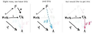
How can we relate the pink and blue lines? We’d really like them to be the same. But we’re in luck because they basically are!
Step 3
H⊆ker(f)H⊆ker(f), that is as long as f(h)=0f(h)=0 for all h∈Hh∈H. And notice that this condition, f(H)=0f(H)=0, forces ff to be RR-balanced!
Let’s check:
Sooooo… homomorphisms f:F→Af:F→A such that H⊆ker(f)H⊆ker(f) are the same as RR-balanced maps from M×NM×N to AA! (Technically, I should say homomorphisms ff restricted to M×NM×N.) In other words, we have
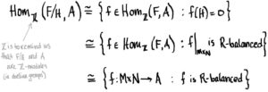
In conclusion, to say “abelian group homomorphisms from F/HF/H to AA are the same as (isomorphic to) RR-balanced maps from M×NM×N to AA” is the simply the hand-wavy way of saying
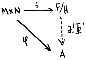
Whenever i:M×N→Fi:M×N→F is an RR-balanced map and φ:M×N→Aφ:M×N→A is an RR-balanced map where AA is an abelian group, there exists a unique abelian group homomorphism Φ:F/H→AΦ:F/H→A such that the following diagram commutes:
And this is just want we want! The last step is merely the final touch:
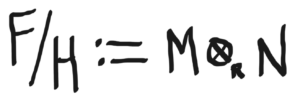
Step 4
the abelian quotient group F/HF/H to be the tensor product of MM and NN,
whose elements are cosets,
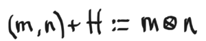
where m⊗nm⊗n for m∈Mm∈M and n∈Nn∈N is referred to as a simple tensor. And there you have it! The tensor product, constructed.
For more such insights, log into www.international-maths-challenge.com.
*Credit for article given to Tai-Danae Bradley*