Category: mathematics

If you want your cup of tea to stay as hot as possible, should you put milk in immediately, or wait until you are ready to drink it? Katie Steckles does the sums.

Picture the scene: you are making a cup of tea for a friend who is on their way and won’t be arriving for a little while. But – disaster – you have already poured hot water onto a teabag! The question is, if you don’t want their tea to be too cold when they come to drink it, do you add the cold milk straight away or wait until your friend arrives?

Luckily, maths has the answer. When a hot object like a cup of tea is exposed to cooler air, it will cool down by losing heat. This is the kind of situation we can describe using a mathematical model – in this case, one that represents cooling. The rate at which heat is lost depends on many factors, but since most have only a small effect, for simplicity we can base our model on the difference in temperature between the cup of tea and the cool air around it.

A bigger difference between these temperatures results in a much faster rate of cooling. So, as the tea and the surrounding air approach the same temperature, the heat transfer between them, and therefore cooling of the tea, slows down. This means that the crucial factor in this situation is the starting condition. In other words, the initial temperature of the tea relative to the temperature of the room will determine exactly how the cooling plays out.

When you put cold milk into the hot tea, it will also cause a drop in temperature. Your instinct might be to hold off putting milk into the tea, because that will cool it down and you want it to stay as hot as possible until your friend comes to drink it. But does this fit with the model?

Let’s say your tea starts off at around 80°C (176°F): if you put milk in straight away, the tea will drop to around 60°C (140°F), which is closer in temperature to the surrounding air. This means the rate of cooling will be much slower for the milky tea when compared with a cup of non-milky tea, which would have continued to lose heat at a faster rate. In either situation, the graph (pictured above) will show exponential decay, but adding milk at different times will lead to differences in the steepness of the curve.

Once your friend arrives, if you didn’t put milk in initially, their tea may well have cooled to about 55°C (131°F) – and now adding milk will cause another temperature drop, to around 45°C (113°F). By contrast, the tea that had milk put in straight away will have cooled much more slowly and will generally be hotter than if the milk had been added at a later stage.

Mathematicians use their knowledge of the rate at which objects cool to study the heat from stars, planets and even the human body, and there are further applications of this in chemistry, geology and architecture. But the same mathematical principles apply to them as to a cup of tea cooling on your table. Listening to the model will mean your friend’s tea stays as hot as possible.

For more such insights, log into www.international-maths-challenge.com.

*Credit for article given to Katie Steckles*

Statistical methods can evaluate whether pivotal military events, like the Battle of Jutland, American involvement in the Vietnam war or the nuclear arms race, could’ve turned out otherwise, according to a new book.

Military historical narratives and statistical modeling bring fresh perspectives to the fore in a ground-breaking text, “Quantifying Counterfactual Military History,” by Brennen Fagan, Ian Horwood, Niall MacKay, Christopher Price and Jamie Wood, a team of historians and mathematicians.

The authors explain, “In writing history, it must always be remembered that a historical fact is simply one of numberless possibilities until the historical actor moves or an event occurs, at which point it becomes real. To understand the one-time possibility that became evidence we must also understand the possibilities that remained unrealized.”

Re-examining the battlefield

Midway through the First World War, Britain and Germany were locked in a technologically driven arms race which culminated in the Battle of Jutland in 1916. By that time, both nations had built over 50 dreadnoughts—speedy, heavily-armored, turbine-powered “all-big-gun” warships.

In the context of a battle that Britain couldn’t afford to lose, Winston Churchill was quoted as saying that the British commander John Jellicoe was “the only man on either side who could lose the war in an afternoon.”

Both nations, at various points in time, have claimed victory in the Battle of Jutland, and there is no consensus on who “won.” Using mathematical modeling, “Quantifying Counterfactual Military History” probes whether the Germans could have achieved a decisive victory.

The five scholars note, “This reconstructive battling enables us to put some level of statistical insight into multiple realizations of a key phase of Jutland. The model is crude and laden with assumptions—as are all wargames—but, unlike in a wargame, our goal is simply to understand what is plausible and what is not.”

Understanding nuclear deterrence

Counterfactual reasoning is positioned centrally when it comes to the fraught history of nuclear deterrence. By the 1980s, the nuclear arms race between the US and the Soviet Union had already spanned three decades and 1983 would bring a crisis less well-known than the Cuban missile crisis of 1962.

The authors draw attention to the peak of intensity in November 1983 during the so-called “Second Cold War.” A NATO “command post” exercise in Western Europe—known as Able Archer—was created to test communications in the event of nuclear war.

The Soviets, however—likely the result of faulty intelligence gathering—believed that an attack was imminent with the NATO exercise interpreted as the first phase. “Quantifying Counterfactual Military History” highlights the example as one where each side placed themselves in dangerous counterfactual mindsets.

“Mutual misapprehension in 1983 continued a long tradition of misunderstanding which had always created catastrophic potential for war, now based consciously and unconsciously on game theory and its erroneous assumption that rational actors were guided by accurate information,” the authors explain. “In this way they stumbled towards a war that neither had willed.”

Embrace the alternative

“Quantifying Counterfactual Military History” uses case studies of Jutland, Able Archer, the Battle of Britain and the Vietnam War to appraise long-established narratives around military events and examine the probabilities of the events that took place alongside the potential for alternative outcomes.

The book’s authors, however, take a restrained approach to counterfactual theory, one that acknowledges and considers why some events—including the actions of individuals or the rise of institutions—are more important than others and can be considered “critical junctures.” They understand this as very different from the arbitrary, loosely substantiated suppositions made by “exuberant” counterfactuals.

They say, “We can never be certain of the existence of critical junctures, or of the grounds of their criticality, but ‘restrained’ counterfactuals, if done with multiple perspectives and sufficient thoroughness, can surely make a distinctive contribution to the literature.”

The book is underpinned by an inter-disciplinary method which combines historical narrative and statistical data and analysis, offering both quantitative and qualitative rigor.

They explain, “This study has taken us in directions which are not common in academic collaboration, but which we hope demonstrate that collaborative research exploring what had been dead ground between the sciences and the humanities is long overdue.”

Rather than attempt to merely reinvent the past, “Quantifying Counterfactual Military History” calls attention to the dynamism inherent in historical practice and offers another tool for understanding historical actors, the decisions they made and the futures they shaped.

For more such insights, log into our website https://international-maths-challenge.com

Credit of the article given to Taylor & Francis

 

Suffixes are important!

Did you know that the words

“maximal” and “maximum” generally do NOT mean the same thing

in mathematics? It wasn’t until I had to think about Zorn’s Lemma in the context of maximal ideals that I actually thought about this, but more on that in a moment. Let’s start by comparing the definitions:

Do you see the difference? An element is a maximum if it is larger than every single element in the set, whereas an element is maximal if it is not smaller than any other element in the set (where “smaller” is determined by the partial order ≤≤). Yes, it’s true that the* maximum also satisfies this property, i.e. every maximum element is also maximal. But the converse is not true: if an element is maximal, it may not be the maximum! Why? The key is that these definitions are made on a partially ordered set. Basically, partially ordered just means it makes sense to use the words “bigger” or “smaller” – we have a way to compare elements. In a totally ordered set ALL elements are comparable with each other. But in a partially ordered set SOME, but not necessarily all, elements can be compared. This means it’s possible to have an element that is maximal yet fails to be the maximum because it cannot be compared with some elements. It’s not too hard to see that when a set is totally ordered, “maximal = maximum.”**

How about an example? Here’s one I like from this scholarly site which also gives an example of a miminal/minimum element (whose definitions are dual to those above).

Example

Consider the set

where the partial order is set inclusion, ⊆⊆. Then

• {d,o}{d,o} is minimalbecause {d,o}⊉x{d,o}⊉x for every x∈Xx∈
• e. there isn’t a single element in XX that is “smaller” than {d,o}{d,o}
• {g,o,a,d}{g,o,a,d} is maximalbecause {g,o,a,d}⊈x{g,o,a,d}⊈x for every x∈Xx∈X
• e. there isn’t a single element in XX that is “larger” than {g,o,a,d}{g,o,a,d}
• {o,a,f}{o,a,f} is both minimal and maximal because
• {o,a,f}⊉x{o,a,f}⊉x for every x∈Xx∈X
• {o,a,f}⊈x{o,a,f}⊈x for every x∈Xx∈X
• {d,o,g}{d,o,g} is neither minimal nor maximal because
• there is an x∈Xx∈X such that x⊆{d,o,g}x⊆{d,o,g}, namely x={d,o}x={d,o}
• there is an x∈Xx∈X such that {d,o,g}⊆x{d,o,g}⊆x, namely x={g,o,a,d}x={g,o,a,d}
• XX has NEITHER a maximum or a minimum because
• there is no M∈XM∈X such that x⊆Mx⊆M for everyx∈Xx∈X
• there is no m∈Xm∈X such that m⊆xm⊆x for everyx∈Xx∈X

Let’s now relate our discussion above to ring theory. One defines an ideal MM in a ring RR to be a maximal ideal if M≠RM≠R and the only ideal that contains MM is either MM or RR itself, i.e. if I⊴RI⊴R is an  ideal such that M⊆I⊆RM⊆I⊆R, then we must have either I=MI=M or I=RI=R.

Not surprisingly, this coincides with the definition of maximality above. We simply let XX be the set of all proper ideals in the ring RR endowed with the partial order of inclusion ⊆⊆. The only difference is that in this context, because we’re in a ring, we have the second option I=RI=R.

I think a good way to see maximal ideals in action is in the proof of this result:

As a final remark, the notions of “a maximal element” and “an upper bound” come together in Zorn’s Lemma which is needed to prove that every proper ideal in a ring is contained in a maximal ideal. I should mention that an upper bound BB on a partially ordered set (a.k.a. a “poset”) has the same definition as the maximum EXCEPT that BB is not required to be inside the set. More precisely, we define an upper bound on a subset YY of XX to be an element B∈XB∈X such that y≤By≤B for every y∈Yy∈Y.

So here’s the deal with Zorn’s Lemma: It’s not too hard to prove that every finite poset has a maximal element. But what if we don’t know if the given poset is finite? Or what happens if it’s infinite? How can we tell if it has a maximal element? Zorn’s Lemma answers that question:

‍As I mentioned above, it’s this result which is needed to prove that every proper ideal is contained in a maximal ideal***. It actually implies a weaker statement, called Krull’s Theorem (1929), which says that every non-zero ring with unity contains a maximal ideal.

‍Footnotes

*One can easily show that if a set has a maximum it must be unique, hence THE maximum.

** Here’s the proof: Let (X,≤)(X,≤) be a totally ordered set and let m∈Xm∈X be a maximal element. It suffices to show mm is the maximum. Since XX has a total order, either m≤xm≤x or x≤mx≤m for every x∈Xx∈X. If the latter, then mm is the maximum. If the former, then m=xm=x by definition of maximal. In either case, we have x≤mx≤m for all x∈Xx∈X. Hence mm is the maximum.

*** Note this is NOT the same as saying that every maximal ideal contains all the proper ideals in a ring! Remember, maximal ≠≠ maximum!!

For more such insights, log into www.international-maths-challenge.com.

*Credit for article given to Tai-Danae Bradley*

Starting with p (p a positive integer) equally distributed dots (vertices) around a circle. Connecting each dot to the next as you move around the circle will give you a regular p-gon – a p-sided polygon with p vertices. If, however, instead of connecting each dot to the one next to it you skip over a fixed number of dots, then you might end up with a star-like pattern, like the ones shown above. In this process, imagine that you start with a particular vertex and move in a counter-clockwise direction. If there are any dots left-over when you get back to the dot you started from, just throw away the unconnected dots.

The Schläfli notation for polygons is very useful for describing regular connected star polygons, and provides an example of how sometimes calculations with notation match exactly with calculations done with diagrams. In this notation, regular polygons like triangle, square, pentagon, etc. are written as {3}, {4}, and {5} respectively. A regular p-gon is written as {p}. If when drawing your p-gon you connect to the second next vertex instead of the first, then you would write this as {p/2}. If you connect to the q’th next vertex, then you would write this polygon as {p/q}. Note that if you are just connecting to the next vertex to make a regular p-gon, this notation gives you {p/1} = {p}, as you would expect.

If you start playing with this process you will notice that {p/q} gives you the same polygon as {p/(p–q)} (as long as you ignore the orientation of the polygon). You may also notice that if q is larger than p, you end up repeating the same patterns, in particular {p/q} = {p/(q mod p)}. Also you will notice that if p and q have common factors, you end up having skipped vertices. In our process we are throwing these away to ensure that our polygons are connected, but you can extend the process and keep them (see note below).

The process described is straightforward to implement in a program. The images shown here were generated in Tinkerplots. To implement it in Tinkerplots, you need two sliders – p and q, and the following attributes:

n = caseIndex()
theta = 2*n*pi(1-q/p)
x = cos(theta)
y = sin(theta)

If you create a plot with y vertical and x horizontal, choose “show connecting lines” and add a filter n<=p+1, you can add a large number of cases to the collection (~200, say) and be able to slide p and q to create a wide variety of connected star polygons. The only restriction is that p must be less than the number of cases you have created. There is nothing special about using Tinkerplots here – any programming environment with reasonable graphics should do a reasonable job (Logo would be fine. :)).

The polygons below are the regular connected polygons based on 12 vertices. Because 12 is divisible by 2, 3, 4, and 6 we end up with regular polygons triangle {3}, square {4}, hexagon {6} and only one star polygon {12/5}. The “degenerate” polygon {2} is known as a “digon.” Here, drawing the diagram first and then seeing what polygon comes out will give you the same result as dividing p/q first and then drawing the corresponding polygon. In this sense, the notation and diagrams nicely reflect each other.

Contrast this with the family of star polygons that are generated when a prime number of vertices are used. The images below are the family of regular connected polygons generated on 13 vertices.

Note – by throwing away the unconnected dots in our process we are ignoring star polygons that are made of overlapping disjoint star or regular polygons, for example two overlapping triangles that make a star of David. These also work well with the Schläfli notation. To create these overlapping polygons, if you have any skipped vertices, you just begin your process again beginning with one of the vertices you skipped over. In the case of {6/2}, instead of getting one triangle {3} you will get two overlapping triangles, or 2{3}. To write a program that would draw these you would want to use something more sophisticated than Tinkerplots.

For more such insights, log into www.international-maths-challenge.com.

*Credit for article given to dan.mackinnon*

Mathematicians are celebrating a 1000-page proof of the geometric Langlands conjecture, a problem so complicated that even other mathematicians struggle to understand it. Despite that, it is hoped the proof can provide key insights across maths and physics.

The Langlands programme aims to link different areas of mathematics

Mathematicians have proved a key building block of the Langlands programme, sometimes referred to as a “grand unified theory” of maths due to the deep links it proposes between seemingly distant disciplines within the field.

While the proof is the culmination of decades of work by dozens of mathematicians and is being hailed as a dazzling achievement, it is also so obscure and complex that it is “impossible to explain the significance of the result to non-mathematicians”, says Vladimir Drinfeld at the University of Chicago. “To tell the truth, explaining this to mathematicians is also very hard, almost impossible.”

The programme has its origins in a 1967 letter from Robert Langlands to fellow mathematician Andre Weil that proposed the radical idea that two apparently distinct areas of mathematics, number theory and harmonic analysis, were in fact deeply linked. But Langlands couldn’t actually prove this, and was unsure whether he was right. “If you are willing to read it as pure speculation I would appreciate that,” wrote Langlands. “If not — I am sure you have a waste basket handy.”

This mysterious link promised answers to problems that mathematicians were struggling with, says Edward Frenkel at the University of California, Berkeley. “Langlands had an insight that difficult questions in number theory could be formulated as more tractable questions in harmonic analysis,” he says.

In other words, translating a problem from one area of maths to another, via Langlands’s proposed connections, could provide real breakthroughs. Such translation has a long history in maths – for example, Pythagoras’s theorem relating the three sides of a triangle can be proved using geometry, by looking at shapes, or with algebra, by manipulating equations.

As such, proving Langlands’s proposed connections has become the goal for multiple generations of researchers and led to countless discoveries, including the mathematical toolkit used by Andrew Wiles to prove the infamous Fermat’s last theorem. It has also inspired mathematicians to look elsewhere for analogous links that might help. “A lot of people would love to understand the original formulation of the Langlands programme, but it’s hard and we still don’t know how to do it,” says Frenkel.

One analogy that has yielded progress is reformulating Langlands’s idea into one written in the mathematics of geometry, called the geometric Langlands conjecture. However, even this reformulation has baffled mathematicians for decades and was itself considered fiendishly difficult to prove.

Now, Sam Raskin at Yale University and his colleagues claim to have proved the conjecture in a series of five papers that total more than 1000 pages. “It’s really a tremendous amount of work,” says Frenkel.

The conjecture concerns objects that are similar to those in one half of the original Langlands programme, harmonic analysis, which describes how complex structures can be mathematically broken down into their component parts, like picking individual instruments out of an orchestra. But instead of looking at these with harmonic analysis, it uses other mathematical ideas, such as sheaves and moduli stacks, that describe concepts relating to shapes like spheres and doughnuts.

While it wasn’t in the setting that Langlands originally envisioned, it is a sign that his original hunch was correct, says Raskin. “Something I find exciting about the work is it’s a kind of validation of the Langlands programme more broadly.”

“It’s the first time we have a really complete understanding of one corner of the Langlands programme, and that’s inspiring,” says David Ben-Zvi at the University of Texas, who wasn’t involved in the work. “That kind of gives you confidence that we understand what its main issues are. There are a lot of subtleties and bells and whistles and complications that appear, and this is the first place where they’ve all been kind of systematically resolved.”

Proving this conjecture will give confidence to other mathematicians hoping to make inroads on the original Langlands programme, says Ben-Zvi, but it might also attract the attention of theoretical physicists, he says. This is because in 2007, physicists Edward Witten and Anton Kapustin found that the geometric Langlands conjecture appeared to describe an apparent symmetry between certain physical forces or theories, called S-duality.

The most basic example of this in the real world is in electricity and magnetism, which are mirror images of one another and interchangeable in many scenarios, but S-duality was also used by Witten to famously unite five competing string theory models into a single theory called M-theory.

But before anything like that, there is much more work to be done, including helping other mathematicians to actually understand the proof. “Currently, there’s a very small group of people who can really understand all the details here. But that changes the game, that changes the whole expectation and changes what you think is possible,” says Ben-Zvi.

For more such insights, log into www.international-maths-challenge.com.

*Credit for article given to Alex Wilkins*

One of the essential skills students need to master in primary school mathematics are “multiplication facts”.

What are they? What are they so important? And how can you help your child master them?

What are multiplication facts?

Multiplication facts typically describe the answers to multiplication sums up to 10×10. Sums up to 10×10 are called “facts” as it is expected they can be easily and quickly recalled. You may recall learning multiplication facts in school from a list of times tables.

The shift from “times tables” to “multiplication facts” is not just about language. It stems from teachers wanting children to see how multiplication facts can be used to solve a variety of problems beyond the finite times table format.

For example, if you learned your times tables in school (which typically went up to 12×12 and no further), you might be stumped by being asked to solve 15×8 off the top of your head. In contrast, we hope today’s students can use their multiplication facts knowledge to quickly see how 15×8 is equivalent to 10×8 plus 5×8.

The shift in terminology also means we are encouraging students to think about the connections between facts. For example, when presented only in separate tables, it is tricky to see how 4×3 and 3×4 are directly connected.

Maths education has changed

In a previous piece, we talked about how mathematics education has changed over the past 30 years.

In today’s mathematics classrooms, teachers still focus on developing students’ mathematical accuracy and fast recall of essential facts, including multiplication facts.

But we also focus on developing essential problem-solving skills. This helps students form connections between concepts, and learn how to reason through a variety of real-world mathematical tasks.

Why are multiplication facts so important?

By the end of primary school, it is expected students will know multiplication facts up to 10×10 and can recall the related division fact (for example, 10×9=90, therefore 90÷10=9).

Learning multiplication facts is also essential for developing “multiplicative thinking”. This is an understanding of the relationships between quantities, and is something we need to know how to do on a daily basis.

When we are deciding whether it is better to purchase a 100g product for $3 or a 200g product for $4.50, we use multiplicative thinking to consider that 100g for $3 is equivalent to 200g for $6 – not the best deal!

Multiplicative thinking is needed in nearly all maths topics in high school and beyond. It is used in many topics across algebra, geometry, statistics and probability.

This kind of thinking is profoundly important. Research showsstudents who are more proficient in multiplicative thinking perform significantly better in mathematics overall.

In 2001, an extensive RMIT study found there can be as much as a seven-year difference in student ability within one mathematics class due to differences in students’ ability to access multiplicative thinking.

These findings have been confirmed in more recent studies, including a 2021 paper.

So, supporting your child to develop their confidence and proficiency with multiplication is key to their success in high school mathematics. How can you help?

Below are three research-based tips to help support children from Year 2 and beyond to learn their multiplication facts.

1. Discuss strategies

One way to help your child’s confidence is to discuss strategies for when they encounter new multiplication facts.

Prompt them to think of facts they already and how they can be used for the new fact.

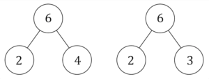
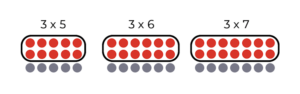
For example, once your child has mastered the x2 multiplication facts, you can discuss how 3×6 (3 sixes) can be calculated by doubling 6 (2×6) and adding one more 6. We’ve now realised that x3 facts are just x2 facts “and one more”!

The Conversation, CC BY-SA

Strategies can be individual: students should be using the strategy that makes the most sense to them. So you could ask a questions such as “if you’ve forgotten 6×7, how could you work it out?” (we might personally think of 6×6=36 and add one more 6, but your child might do something different and equally valid).

This is a great activity for any quiet car trip. It can also be a great drawing activity where you both have a go at drawing your strategy and then compare. Identifying multiple strategies develops flexible thinking.

2. Help them practise

Practising recalling facts under a friendly time crunch can be helpful in achieving what teachers call “fluency” (that is, answering quickly and easily).

A great game you could play with your children is “multiplication heads up” . Using a deck of cards, your child places a card to their forehead where you can see but they cannot. You then flip over the top card on the deck and reveal it to your child. Using the revealed card and the card on your child’s head you tell them the result of the multiplication (for example, if you flip a 2 and they have a 3 card, then you tell them “6!”).

Based on knowing the result, your child then guesses what their card was.

If it is challenging to organise time to pull out cards, you can make an easier game by simply quizzing your child. Try to mix it up and ask questions that include a range of things they know well with and ones they are learning.

Repetition and rehearsal will mean things become stored in long-term memory.

3. Find patterns

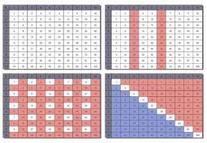
Another great activity to do at home is print some multiplication grids and explore patterns with your child.

The Conversation, CC BY-SA

A first start might be to give your child a blank or partially blankmultiplication grid which they can practise completing.

Then, using coloured pencils, they can colour in patterns they notice. For example, the x6 column is always double the answer in the x3 column. Another pattern they might see is all the even answers are products of 2, 4, 6, 8, 10. They can also notice half of the grid is repeated along the diagonal.

This also helps your child become a mathematical thinker, not just a calculator.

The importance of multiplication for developing your child’s success and confidence in mathematics cannot be understated. We believe these ideas will give you the tools you need to help your child develop these essential skills.

For more such insights, log into our website https://international-maths-challenge.com

 

From the Fibonacci sequence to the Bell numbers, there is more overlap between mathematics and poetry than you might think, says Peter Rowlett, who has found his inner poet.

People like to position maths as cold, hard logic, quite distinct from creative pursuits. Actually, maths often involves a great deal of creativity. As mathematician Sofya Kovalevskaya wrote, “It is impossible to be a mathematician without being a poet in soul.” Poetry is often constrained by rules, and these add to, rather than detract from, its creativity.

Rhyming poems generally follow a scheme formed by giving each line a letter, so that lines with matching letters rhyme. This verse from a poem by A. A. Milne uses an ABAB scheme:

What shall I call
My dear little dormouse?
His eyes are small,
But his tail is e-nor-mouse.

In poetry, as in maths, it is important to understand the rules well enough to know when it is okay to break them. “Enormous” doesn’t rhyme with “dormouse”, but using a nonsense word preserves the rhyme while enhancing the playfulness.

There are lots of rhyme schemes. We can count up all the possibilities for any number of lines using what are known as the Bell numbers. These count the ways of dividing up a set of objects into smaller groupings. Two lines can either rhyme or not, so AA and AB are the only two possibilities. With three lines, we have five: AAA, ABB, ABA, AAB, ABC. With four, there are 15 schemes. And for five lines there are 52 possible rhyme schemes!

Maths is also at play in Sanskrit poetry, in which syllables have different weights. “Laghu” (light) syllables take one unit of metre to pronounce, and “guru” (heavy) syllables take two units. There are two ways to arrange a line of two units: laghu-laghu, or guru. There are three ways for a line of three units: laghu-laghu-laghu; laghu-guru; and guru-laghu. For a line of four units, we can add guru to all the ways to arrange two units or add laghu to all the ways to arrange three units, yielding five possibilities in total. As the number of arrangements for each length is counted by adding those of the previous two, these schemes correspond with Fibonacci numbers.

Not all poetry rhymes, and there are many ways to constrain writing. The haiku is a poem of three lines with five, seven and five syllables, respectively – as seen in an innovative street safety campaign in New York City, above.

Some creative mathematicians have come up with the idea of a π-ku (pi-ku) based on π, which can be approximated as 3.14. This is a three-line poem with three syllables on the first line, one on the second and four on the third. Perhaps you can come up with your own π-ku – here is my attempt, dreamt up in the garden:

White seeds float,
dance,
spinning around.

For more such insights, log into www.international-maths-challenge.com.

*Credit for article given to Peter Rowlett

Looking at the last few digits that appear in the numbers that form the sequence b^0, b^1, b^2, b^3, … for b a positive integer, you’ll notice that the digits will always begin to repeat after a certain point. For example, looking at the last digit of the sequences for b = 2, 3, and 4 we have the sequences

b = 2: 1, 2, 4, 8, 6, 2, 4, 8, 6, …
b = 3: 1, 3, 9, 7, 1, 3, 9, 7, …
b = 4: 1, 4, 6, 4, 6, 4, 6, …

If we look at the sequence of last two digits of these sequence where b =2 we have

b = 2: 1, 2, 4, 8, 16, 32, 64, 28, 56, 12, 24, 48, 96, 92, 84, 68, 36, 72, 44, 88, 76, 52, 4, …

This sequence then repeats the loop that began at 4.

We can describe these sequences as T_b,d(n) = (b^n)mod 10^d. Recursively, T_b,d(n) = (T_b,d(n-1)*b)mod 10^d

These sequences are always eventually periodic. Although these sequences are simple to understand and calculate, there are several interesting ways of describing them.

For example, you can think of the elements of T_b,d as a commutative monoid, with multiplication defined as a*b = (a*b)mod 10^d. They form a monoid since 1 is always a member, and you can show that T_b,d is closed under the * operation. It turns out that for some values of b, and d, T_b,d is a group.

You can also think of this set as a finite state machine or graph, where each element is a node and the transition from one node to the next is defined by the operation *b mod 10^d. This provides a nice way of displaying the sequences. The pictures in this post were created by writing a short program to calculate the sequences, and then formatting the output to draw a di-graph in SAGE. The graph at the top of the post is for b=8, d=1, while the graph below is for b=2, d=2. The graph at the bottom of the page is for b=7, d=1.

For more such insights, log into www.international-maths-challenge.com.

*Credit for article given to dan.mackinnon*

Felker prefaces the quote by saying,

Giving up on math means you don’t believe that careful study can change the way you think.

He further notes that writing, like math, “is also not something that anyone is ‘good’ at without a lot of practice, but it would be completely unacceptable to think that your composition skills could not improve.”

Friends, this is so true! Being ‘good’ at math boils down to hard work and perseverance, not whether or not you have the ‘math gene.’ “But,” you might protest, “I’m so much slower than my classmates are!” or “My educational background isn’t as solid as other students’!” or “I got a late start in mathematics!”* That’s okay! A strong work ethic and a love and enthusiasm for learning math can shore up all deficiencies you might think you have. Now don’t get me wrong. I’m not claiming it’ll be a walk in the park. To be honest, some days it feels like a walk through an unfamiliar alley at nighttime during a thunderstorm with no umbrella. But, you see, that’s okay too. It may take some time and the road may be occasionally bumpy, but it can be done!

This brings me to another point that Felker makes: If you enjoy math but find it to be a struggle, do not be discouraged! The field of math is HUGE and its subfields come in many different flavors. So for instance, if you want to be a math major but find your calculus classes to be a challenge, do not give up! This is not an indication that you’ll do poorly in more advanced math courses. In fact, upper level math classes have a completely (I repeat, completely!) different flavor than calculus. Likewise, in graduate school you may struggle with one course, say algebraic topology, but find another, such as logic, to be a breeze. Case in point: I loathed real analysis as an undergraduate** and always thought it was pretty masochistic. But real analysis in graduate school was nothing like undergraduate real analysis (which was more like advanced calculus), and now – dare I say it? – I sort of enjoy the subject. (Gasp!)

All this to say that although Felker’s article is aimed at folks who may be afraid to take college-level math, I think it applies to math majors and graduate students too. I highly recommend you read it if you ever need a good ‘pick-me-up.’ And on those days when you feel like the math struggle is harder than usual, just remember:

Even the most accomplished mathematicians had to learn HOW to learn this stuff!

For more such insights, log into www.international-maths-challenge.com.

*Credit for article given to Tai-Danae Bradley*

A mathematical model of a particle that remembers its past so that it never travels the same path twice produces stunningly complex patterns.

A beautiful and surprisingly complex pattern produced by ‘mathematical billiards’

Albers et al. PRL 2024

In a mathematical version of billiards, particles that avoid retracing their paths get trapped in intricate and hard-to-predict patterns – which might eventually help us understand the complex movement patterns of living organisms.

When searching for food, animals including ants and slime moulds leave chemical trails in their environment, which helps them avoid accidentally retracing their steps. This behaviour is not uncommon in biology, but when Maziyar Jalaal at the University of Amsterdam in the Netherlands and his colleagues modelled it as a simple mathematical problem, they uncovered an unexpected amount of complexity and chaos.

They used the framework of mathematical billiards, where an infinitely small particle bounces between the edges of a polygonal “table” without friction. Additionally, they gave the particle “spatial memory” – if it reached a point where it had already been before, it would reflect off it as if there was a wall there.

The researchers derived equations describing the motion of the particle and then used them to simulate this motion on a computer. They ran over 200 million simulations to see the path the particle would take inside different polygons – like a triangle and a hexagon – over time. Jalaal says that though the model was simple, idealised and deterministic, what they found was extremely intricate.

Within each polygon, the team identified regions where the particle was likely to become trapped after bouncing around for a long time due to its “remembering” its past trajectories, but zooming in on those regions revealed yet more patterns of motion.

“So, the patterns that you see if you keep zooming in, there is no end to them. And they don’t repeat, they’re not like fractals,” says Jalaal.

Katherine Newhall at the University of North Carolina at Chapel Hill says the study is an “interesting mental exercise” but would have to include more detail to accurately represent organisms and objects that have spatial memory in the real world. For instance, she says that a realistic particle would eventually travel in an imperfectly straight line or experience friction, which could radically change or even eradicate the patterns that the researchers found.

For more such insights, log into www.international-maths-challenge.com.

*Credit for article given to Karmela Padavic-Callaghan*