Category: mathematics

Does the thought of p-values and regressions make you break out in a cold sweat? Never fear – read on for answers to some of those burning statistical questions that keep you up 87.9% of the night.

• What are my hypotheses?

There are two types of hypothesis you need to get your head around: null and alternative. The null hypothesis always states the status quo: there is no difference between two populations, there is no effect of adding fertiliser, there is no relationship between weather and growth rates.

Basically, nothing interesting is happening. Generally, scientists conduct an experiment seeking to disprove the null hypothesis. We build up evidence, through data collection, against the null, and if the evidence is sufficient we can say with a degree of probability that the null hypothesis is not true.

We then accept the alternative hypothesis. This hypothesis states the opposite of the null: there is a difference, there is an effect, there is a relationship.

• What’s so special about 5%?

One of the most common numbers you stumble across in statistics is alpha = 0.05 (or in some fields 0.01 or 0.10). Alpha denotes the fixed significance level for a given hypothesis test. Before starting any statistical analyses, along with stating hypotheses, you choose a significance level you’re testing at.

This states the threshold at which you are prepared to accept the possibility of a Type I Error – otherwise known as a false positive – rejecting a null hypothesis that is actually true.

• Type what error?

Most often we are concerned primarily with reducing the chance of a Type I Error over its counterpart (Type II Error – accepting a false null hypothesis). It all depends on what the impact of either error will be.

Take a pharmaceutical company testing a new drug; if the drug actually doesn’t work (a true null hypothesis) then rejecting this null and asserting that the drug does work could have huge repercussions – particularly if patients are given this drug over one that actually does work. The pharmaceutical company would be concerned primarily with reducing the likelihood of a Type I Error.

Sometimes, a Type II Error could be more important. Environmental testing is one such example; if the effect of toxins on water quality is examined, and in truth the null hypothesis is false (that is, the presence of toxins does affect water quality) a Type II Error would mean accepting a false null hypothesis, and concluding there is no effect of toxins.

The down-stream issues could be dire, if toxin levels are allowed to remain high and there is some health effect on people using that water.

Do you know the difference between continuous and categorical variables?

• What is a p-value, really?

Because p-values are thrown about in science like confetti, it’s important to understand what they do and don’t mean. A p-value expresses the probability of getting a given result from a hypothesis test, or a more extreme result, if the null hypothesis were true.

Given we are trying to reject the null hypothesis, what this tells us is the odds of getting our experimental data if the null hypothesis is correct. If the odds are sufficiently low we feel confident in rejecting the null and accepting the alternative hypothesis.

What is sufficiently low? As mentioned above, the typical fixed significance level is 0.05. So if the probability portrayed by the p-value is less than 5% you reject the null hypothesis. But a fixed significance level can be deceiving: if 5% is significant, why is 6% not?

It pays to remember that such probabilities are continuous, and any given significance level is arbitrary. In other words, don’t throw your data away simply because you get a p-value of 6-10%.

• How much replication do I have?

This is probably the biggest issue when it comes to experimental design, in which the focus is on ensuring the right type of data, in large enough quantities, is available to answer given questions as clearly and efficiently as possible.

Pseudoreplication refers to the over-inflation of degrees of freedom (a mathematical restriction put in place when we calculate a parameter – e.g. a mean – from a sample). How would this work in practice?

Say you’re researching cholesterol levels by taking blood from 20 male participants.

Each male is tested twice, giving 40 test results. But the level of replication is not 40, it’s actually only 20 – a requisite for replication is that each replicate is independent of all others. In this case, two blood tests from the same person are intricately linked.

If you were to analyse the data with a sample size of 40, you would be committing the sin of pseudoreplication: inflating your degrees of freedom (which incidentally helps to create a significant test result). Thus, if you start an experiment understanding the concept of independent replication, you can avoid this pitfall.

• How do I know what analysis to do?

There is a key piece of prior knowledge that will help you determine how to analyse your data. What kind of variable are you dealing with? There are two most common types of variable:

1) Continuous variables. These can take any value. Were you to you measure the time until a reaction was complete, the results might be 30 seconds, two minutes and 13 seconds, or three minutes and 50 seconds.

2) Categorical variables. These fit into – you guessed it – categories. For instance, you might have three different field sites, or four brands of fertiliser. All continuous variables can be converted into categorical variables.

With the above example we could categorise the results into less than one minute, one to three minutes, and greater than three minutes. Categorical variables cannot be converted back to continuous variables, so it’s generally best to record data as “continuous” where possible to give yourself more options for analysis.

Deciding which to use between the two main types of analysis is easy once you know what variables you have:

ANOVA (Analysis of Variance) is used to compare a categorical variable with a continuous variable – for instance, fertiliser treatment versus plant growth in centimetres.

Linear Regression is used when comparing two continuous variables – for instance, time versus growth in centimetres.

Though there are many analysis tools available, ANOVA and linear regression will get you a long way in looking at your data. So if you can start by working out what variables you have, it’s an easy second step to choose the relevant analysis.

Ok, so perhaps that’s not everything you need to know about statistics, but it’s a start. Go forth and analyse!

For more such insights, log into www.international-maths-challenge.com.

*Credit for article given to Sarah-Jane O’Connor*

 

Elliptic curves have a long and distinguished history that can be traced back to antiquity. They are prevalent in many branches of modern mathematics, foremost of which is number theory.

In simplest terms, one can describe these curves by using a cubic equation of the form

where A and B are fixed rational numbers (to ensure the curve E is nice and smooth everywhere, one also needs to assume that its discriminant 4A³ + 27B² is non-zero).

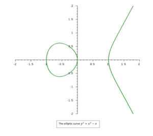
To illustrate, let’s consider an example: choosing A=-1 and B=0, we obtain the following picture:

At this point it becomes clear that, despite their name, elliptic curves have nothing whatsoever to do with ellipses! The reason for this historical confusion is that these curves have a strong connection to elliptic integrals, which arise when describing the motion of planetary bodies in space.

The ancient Greek mathematician Diophantus is considered by many to be the father of algebra. His major mathematical work was written up in the tome Arithmetica which was essentially a school textbook for geniuses. Within it, he outlined many tools for studying solutions to polynomial equations with several variables, termed Diophantine Equations in his honour.

One of the main problems Diophantus considered was to find all solutions to a particular polynomial equation that lie in the field of rational numbers Q. For equations of “degree two” (circles, ellipses, parabolas, hyperbolas) we now have a complete answer to this problem. This answer is thanks to the late German mathematician Helmut Hasse, and allows one to find all such points, should they exist at all.

Returning to our elliptic curve E, the analogous problem is to find all the rational solutions (x,y) which satisfy the equation defining E. If we call this set of points E(Q), then we are asking if there exists an algorithm that allows us to obtain all points (x,y) belonging to E(Q).

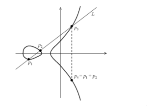
At this juncture we need to introduce a group law on E, which gives an eccentric way of fusing together two points (p₁ and p₂) on the curve, to obtain a brand new point (p₄). This mimics the addition law for numbers we learn from childhood (i.e. the sum or difference of any two numbers is still a number). There’s an illustration of this rule below:

Under this geometric model, the point p₄ is defined to be the sum of p₁ and p₂ (it’s easy to see that the addition law does not depend on the order of the points p₁, p₂). Moreover the set of rational points is preserved by this notion of addition; in other words, the sum of two rational points is again a rational point.

Louis Mordell, who was Sadleirian Professor of Pure Mathematics at Cambridge University from 1945 to 1953, was the first to determine the structure of this group of rational points. In 1922 he proved

where the number of copies of the integers Z above is called the “rank r(E) of the elliptic curve E”. The finite group Τ_E(Q) on the end is uninteresting, as it never has more than 16 elements.

For more such insights, log into www.international-maths-challenge.com.

*Credit for article given to Daniel Delbourgo*

I work on the mathematics of sharing resources, which has led me to consider emotions such as envy, behaviour such as risk-taking and the best way to cut a cake.

Like, I suspect, many women, my wife enjoys eating dessert but not ordering it. I therefore dutifully order what I think she’ll like, cut it in half and invite her to choose a piece.

This is a sure-fire recipe for marital accord. Indeed, many mathematicians, economists, political scientists and others have studied this protocol and would agree. The protocol is known as the “cut-and-choose” procedure. I cut. You choose.

Cut-and-choose

Cut-and-choose is not limited to the dining table – it dates back to antiquity. It appears nearly 3,000 years ago in Hesiod’s poem Theogeny where Prometheus divides a cow and Zeus selects the part he prefers.

In more recent times, cut-and-choose has been enshrined in the UN’s 1982 Convention of the Law of the Sea where it was proposed as a mechanism to resolve disputes when dividing the seabed for mining.

To study the division of cake, cows and the seabed in a more formal way, various mathematical models have been developed. As with all models, these need to make a number of simplifying assumptions.

One typical assumption is that the people employing the cut-and-choose method are risk-averse. They won’t adopt a risky strategy that may give them less cake than a more conservative strategy.

With such assumptions in place, we can then prove what properties cake cutting procedures have and don’t have. For instance, cut-and-choose is envy free.

You won’t envy the cake I have, otherwise you would have taken this piece. And I won’t envy the piece you have, as the only risk-averse strategy is for me to cut the cake into two parts that I value equally.

On the other hand, the cutting of the cake is not totally equitable since the player who chooses can get cake that has more than half the total value for them.

With two players, it’s hard to do better than cut-and-choose. But I should record that my wife argues with me about this.

She believes it favours the second player since the first player inevitably can’t divide the cake perfectly and the second player can capitalise on this. This is the sort of assumption ignored in our mathematical models.

My wife might prefer the moving-knife procedure which doesn’t favour either player. A knife is moved over the cake, and either player calls “cut” when they are happy with the slice.

Again, this will divide the cake in such a way that neither player will envy the other (else they would have called “cut” themselves).

Three’s a crowd

Unfortunately, moving beyond two players increases the complexity of cutting cake significantly.

With two players, we needed just one cut to get to an envy free state. With three players, a complex series of five cuts of the cake might be needed. Of course, only two cuts are needed to get three slices.

The other three cuts are needed to remove any envy. And with four players, the problem explodes in our face.

An infinite number of cuts may be required to get to a situation where no one envies another’s cake. I’m sure there’s some moral here about too many cake cutters spoiling the dessert.

There are many interesting extensions of the problem. One such extension is to indivisible goods.

Suppose you have a bag of toys to divide between two children. How do you divide them fairly? As a twin myself, I know that the best solution is to ensure you buy two of everything.

It’s much more difficult when your great aunt gives you one Zhu Zhu pet, one Bratz doll and three Silly Bandz bracelets to share.

Online

More recently, I have been studying a version of the problem applicable to online settings. In such problems, not all players may be available all of the time. Consider, for instance, allocating time on a large telescope.

Astronomers will have different preferences for when to use the telescope depending on what objects are visible, the position of the sun, etcetera. How do we design a web-based reservation system so that astronomers can choose observation times that is fair to all?

We don’t want to insist all astronomers log in at the same time to decide an allocation. And we might have to start allocating time on the telescope now, before everyone has expressed their preferences. We can view this as a cake-cutting problem where the cake is made up of the time slots for observations.

The online nature of such cake-cutting problems poses some interesting new challenges.

How can we ensure that late-arriving players don’t envy cake already given to earlier players? The bad news is that we cannot now achieve even a simple property like envy freeness.

No procedure can guarantee situations where players don’t envy one another. But more relaxed properties are possible, such as not envying cake allocated whilst you are participating in the cutting of the cake.

Ham sandwich

There’s a brilliantly named piece of mathematics due to Arthur H. Stone and [John Tukey](http://www.morris.umn.edu/~sungurea/introstat/history/w98/Tukey.html, the Ham Sandwich Theorem which proves we can always cut a three-layered cake perfectly with a single cut.

Suppose we have three objects. Let’s call them “the top slice of bread”, “the ham filling” and “the bottom slice of bread”. Or if you prefer “the top layer” of the cake, “the middle layer” and “the bottom layer”.

The ham sandwich theorem proves a single slice can always perfectly bisect the three objects. Actually, the ham sandwich theorem works in any number of dimensions: any n objects in n-dimensional space can be simultaneously bisected by a single (n − 1) dimensional hyperplane.

So, in the case of the three-layered cake, n = 3, and the three-layered cake can be bisected (or cut) using a single, two-dimensional “hyperplane”. Such as, say, a knife.

Who would have thought that cutting cake would lead to higher dimensions of mathematics by way of a ham sandwich?

For more such insights, log into www.international-maths-challenge.com.

*Credit for article given to Toby Walsh*

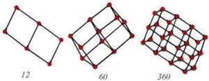
The objects pictured above are interesting structures – they are derived from the prime factorization of a given number n. They can be described in a number of ways – for example, as directed graphs. Because they are nicely structured, they actually form something more special – a lattice. Accordingly, these structures are called factor lattices.
It’s easy to start drawing these by hand following the instructions below.

1. The first node is 1
2. Draw arrows out of this node for each of the prime factors of n.
3. The arrows that you just drew should connect to nodes labled with the prime factors of n.

Now, for each of the new nodes that you drew do the following:

4. Start from a node x that is not equal to n.
5. Draw arrows out of this node for each of the prime factors of n/x.
6. The arrows that you just drew (one for each p = n/x) should connect to nodes labled with the numbers p*x.

7. Now repeat 4,5, and 6 for each new node that you have drawn that is not equal to n.

This process is recursive, and ends when you have the complete lattice. The process is well suited for implementation as a computer program – the images above were created using SAGE using output from a Java program based on the algorithm above.

Manually trying out the steps out for a number like n = 24 goes something like this: First write out the prime factorization of 24, 24=(2*2*2)*3 = (2^3)*3. Starting with 1, draw arrows out to 2 and 3. Now looking at each node and following the algorithm, from the 2 you will get arrows out to 4 and 6. From the 3 you will get an arrow out to 6 as well. From 4 you will get arrows out to 8 or 12. From 6 you will get an arrow out to 12 as well. From 8 and from 12 you get arrows out to 24, and you are done.

In general, the algorithm produces a lattice that can be described as follows. Each node is a factor of the given number n. Two nodes are connected by an edge if their prime factorization differs by a single prime number. In other words, if a and b are nodes, and p = b/a, then there is an arrow p:a–>b.

It’s a good exercise to make the connections between the lattice structure and the prime factorization of a number n.

1. What does the factor lattice of a prime number look like?
2. If a number is just a power of a prime, what does its lattice look like?
3. If you know the factorization, can you find the number of nodes without drawing the lattice.

The answer to the last question (3) can be expressed as:

For example, if n = 24= 2^3*3, then the number of nodes will be (3+1)(1+1) = 8

That these structures can be thought of as “lattices”comes from the fact that you can think of the arrows as an ordering of the nodes, ab. The number 1 is always the least node in the factor lattice for n, while n itself is the greatest node. The property that actually makes these structures a “lattice” is that for any two nodes there is always a lower-bound for any pair of nodes in the lattice, and always an upper-bound for the pair (these are often referred to as meets and joins).

The Wolfram Demonstrations Project has a nice factor lattice demo that will draw factor lattices for a large number of integers for you. There is also a good Wikipedia entry for lattices in general.

For more such insights, log into www.international-maths-challenge.com.

*Credit for article given to dan.mackinnon*

 

While adding up your grocery bill in the supermarket, you’re probably not thinking how important or sophisticated our number system is.

But the discovery of the present system, by unknown mathematicians in India roughly 2,000 years ago – and shared with Europe from the 13th century onwards – was pivotal to the development of our modern world.

Now, what if our “decimal” arithmetic, often called the Indo-Arabic system, had been discovered earlier? Or what if it had been shared with the Western world earlier than the 13th century?

First, let’s define “decimal” arithmetic: we’re talking about the combination of zero, the digits one through nine, positional notation, and efficient rules for arithmetic.

“Positional notation” means that the value represented by a digit depends both on its value and position in a string of digits.

Thus 7,654 means:

(7 × 1000) + (6 × 100) + (5 × 10) + 4 = 7,654

The benefit of this positional notation system is that we need no new symbols or calculation schemes for tens, hundreds or thousands, as was needed when manipulating Roman numerals.

While numerals for the counting numbers one, two and three were seen in all ancient civilisations – and some form of zero appeared in two or three of those civilisations (including India) – the crucial combination of zero and positional notation arose only in India and Central America.

Importantly, only the Indian system was suitable for efficient calculation.

Positional arithmetic can be in base-ten (or decimal) for humans, or in base-two (binary) for computers.

In binary, 10101 means:

(1 × 16) + (0 × 8) + (1 × 4) + (0 × 2) + 1

Which, in the more-familiar decimal notation, is 21.

The rules we learned in primary school for addition, subtraction, multiplication and division can be easily extended to binary.

The binary system has been implemented in electronic circuits on computers, mostly because the multiplication table for binary arithmetic is much simpler than the decimal system.

Of course, computers can readily convert binary results to decimal notation for us humans.

As easy as counting from one to ten

Perhaps because we learn decimal arithmetic so early, we consider it “trivial”.

Indeed the discovery of decimal arithmetic is given disappointingly brief mention in most western histories of mathematics.

In reality, decimal arithmetic is anything but “trivial” since it eluded the best minds of the ancient world including Greek mathematical super-genius Archimedes of Syracuse.

Archimedes – who lived in the 3rd century BCE – saw far beyond the mathematics of his time, even anticipating numerous key ideas of modern calculus. He also used mathematics in engineering applications.

Nonetheless, he used a cumbersome Greek numeral system that hobbled his calculations.

Imagine trying to multiply the Roman numerals XXXI (31) and XIV (14).

First, one must rewrite the second argument as XIIII, then multiply the second by each letter of the first to obtain CXXXX CXXXX CXXXX XIIII.

These numerals can then be sorted by magnitude to arrive at CCCXXXXXXXXXXXXXIIII.

This can then be rewritten to yield CDXXXIV (434).

(For a bit of fun, try adding MCMLXXXIV and MMXI. First person to comment with the correct answer and their method gets a jelly bean.)

Thus, while possible, calculation with Roman numerals is significantly more time-consuming and error prone than our decimal system (although it is harder to alter the amount payable on a Roman cheque).

History lesson

Although decimal arithmetic was known in the Arab world by the 9th century, it took many centuries to make its way to Europe.

Italian mathematician Leonardo Fibonacci travelled the Mediterranean world in the 13th century, learning from the best Arab mathematicians of the time. Even then, it was several more centuries until decimal arithmetic was fully established in Europe.

Johannes Kepler and Isaac Newton – both giants in the world of physics – relied heavily on extensive decimal calculations (by hand) to devise their theories of planetary motion.

In a similar way, present-day scientists rely on massive computer calculations to test hypotheses and design products. Even our mobile phones do surprisingly sophisticated calculations to process voice and video.

But let us indulge in some alternate history of mathematics. What if decimal arithmetic had been discovered in India even earlier, say 300 BCE? (There are indications it was known by this date, just not well documented.)

And what if a cultural connection along the silk-road had been made between Indian mathematicians and Greek mathematicians at the time?

Such an exchange would have greatly enhanced both worlds, resulting in advances beyond the reach of each system on its own.

For example, a fusion of Indian arithmetic and Greek geometry might well have led to full-fledged trigonometry and calculus, thus enabling ancient astronomers to deduce the laws of motion and gravitation nearly two millennia before Newton.

In fact, the combination of mathematics, efficient arithmetic and physics might have accelerated the development of modern technology by more than two millennia.

It is clear from history that without mathematics, real progress in science and technology is not possible (try building a mobile phone without mathematics). But it’s also clear that mathematics alone is not sufficient.

The prodigious computational skills of ancient Indian mathematicians never flowered into advanced technology, nor did the great mathematical achievements of the Greeks, or many developments in China.

On the other hand, the Romans, who were not known for their mathematics, still managed to develop some impressive technology.

But a combination of advanced mathematics, computation, and technology makes a huge difference.

Our bodies and our brains today are virtually indistinguishable from those of ancient times.

With the earlier adoption of Indo-Arabic decimal arithmetic, the modern technological world of today might – for better or worse – have been achieved centuries ago.

And that’s something worth thinking about next time you’re out grocery shopping.

For more such insights, log into www.international-maths-challenge.com.

*Credit for article given to Jonathan Borwein (Jon)*

Could a system of eight-dimensional numbers help physicists find a single mathematical framework that describes the entire universe?

Words can be slippery. That is perhaps even more true in physics than it is in the rest of life. Think of a “particle”, for instance, and we might conjure an image of a tiny sphere. In truth, “particle” is just a poetic term for something far removed from our everyday experience – which is why our best descriptions of reality make use of the cold precision of mathematics.

But just as there are many human languages, so there is more than one type of number system. Most of us deal with only the familiar number line that begins 1, 2, 3. But other, more exotic systems are available. Recently, physicists have been asking a profound question: what if we are trying to describe reality with the wrong type of numbers?

Each mathematical system has its own special disposition, just like languages. Love poems sound better in French. German has that knack of expressing sophisticated concepts – like schadenfreude – in a few syllables. Now, in the wake of a fresh breakthrough revealing tantalising connections between models of how matter works at different energy scales, it seems increasingly likely that an exotic set of numbers known as the octonions might have what it takes to capture the truth about reality.

Mathematicians are excited because they reckon that by translating our theories of reality into the language of the octonions, it could tidy up some of the deepest problems in physics and clear a path to a “grand unified theory” that can describe the universe in one statement. “This feels like a very promising direction,” says Latham Boyle at the Perimeter Institute in Waterloo, Canada. “I find it irresistible to think about.”

Many physicists dream of finding a grand unified theory, a single mathematical framework that tells us where the forces of nature come from and how they act on matter. Critically, such a theory would also capture how and why these properties changed over the life of the universe, as we know they have.

So far, the closest we have come is the standard model of particle physics, which details the universe’s fundamental particles and forces: electrons, quarks, photons and the rest. The trouble is, the standard model has its shortcomings. To make it work, we must feed in around 20 measured numbers, such as the masses of particles. We don’t know why these numbers are what they are. Worse, the standard model has little to say about space-time, the canvas in which particles live. We seem to live in a four-dimensional space-time, but the standard model doesn’t specify that this must be so. “Why not, say, seven-dimensional space-time?” Boyle wonders.

Real and imaginary numbers

Many think the solution to these woes will come when experiments uncover a missing piece of the standard model. But after years of effort, this hasn’t happened, and some are wondering if the problem is the maths itself.

Mathematicians have known for centuries that there are numbers other than the ones we can count on our fingers. Take the square root of -1, known as i. There is no meaningful answer to this expression, as both 1 × 1 and -1 × -1 are equal to 1, so i is an “imaginary number”. They found that by combining i with real numbers – which include all the numbers you could place on a number line, including negative numbers and decimals – they could fashion a new system called the complex numbers.

Think of complex numbers as being two-dimensional; the two parts of each number can record unrelated properties of the same object. This turns out to be extremely handy. All our electronic infrastructure relies on complex numbers. And quantum theory, our hugely successful description of the small-scale world, doesn’t work without them.

In 1843, Irish mathematician William Rowan Hamilton took things a step further. Supplementing the real and the imaginary numbers with two more sets of imaginary numbers called j and k, he gave us the quaternions, a set of four-dimensional numbers. Within a few months, Hamilton’s friend John Graves had found another system with eight dimensions called the octonions.

Real numbers, complex numbers, quarternions and octonions are collectively known as the normed division algebras. They are the only sets of numbers with which you can perform addition, subtraction, multiplication and division. Wilder systems are possible – the 16-dimensional sedenions, for example – but here the normal rules break down.

Today, physics makes prolific use of three of these systems. The real numbers are ubiquitous. Complex numbers are essential in particle physics as well as quantum physics. The mathematical structure of general relativity, Albert Einstein’s theory of gravity, can be expressed elegantly by the quaternions.

The octonions stand oddly apart as the only system not to tie in with a central physical law. But why would nature map onto only three of these four number systems? “This makes one suspect that the octonions – the grandest and least understood of the four – should turn out to be important too,” says Boyle.

In truth, physicists have been thinking such thoughts since the 1970s, but the octonions have yet to fulfil their promise. Michael Duff at Imperial College London was, and still is, drawn to the octonions, but he knows many have tried and failed to decipher their role in describing reality. “The octonions became known as the graveyard of theoretical physics,” he says.

That hasn’t put off a new generation of octonion wranglers, including Nichol Furey at Humboldt University of Berlin. She likes to look at questions in physics without making any assumptions. “I try to solve problems right from scratch,” she says. “In doing so, you can often find alternate paths that earlier authors may have missed.” Now, it seems she and others might be making the beginnings of an octonion breakthrough.

Internal symmetries in quantum mechanics

To get to grips with Furey’s work, it helps to understand a concept in physics called internal symmetry. This isn’t the same as the rotational or reflectional symmetry of a snowflake. Instead, it refers to a number of more abstract properties, such as the character of certain forces and the relationships between fundamental particles. All these particles are defined by a series of quantum numbers – their mass, charge and a quantum property called spin, for instance. If a particle transforms into another particle – an electron becoming a neutrino, say – some of those numbers will change while others won’t. These symmetries define the structure of the standard model.

Internal symmetries are central to the quest for a grand unified theory. Physicists have already found various mathematical models that might explain how reality worked back at the time when the universe had much more energy. At these higher energies, it is thought there would have been more symmetries, meaning that some forces we now experience as distinct would have been one and the same. None of these models have managed to rope gravity into the fold: that would require an even grander “theory of everything”. But they do show, for instance, that the electromagnetic force and weak nuclear force would have been one “electroweak” force until a fraction of a second after the big bang. As the universe cooled, some of the symmetries broke, meaning this particular model would no longer apply.

Each different epoch requires a different mathematical model with a gradually reducing number of symmetries. In a sense, these models all contain each other, like a set of Russian dolls.

One of the most popular candidates for the outermost doll – the grand unified theory that contains all the others – is known as the spin(10) model. It has a whopping 45 symmetries. In one formulation, inside this sits the Pati-Salam model, with 21 symmetries. Then comes the left-right symmetric model, with 15 symmetries, including one known as parity, the kind of left-right symmetry that we encounter when we look in a mirror. Finally, we reach the standard model, with 12 symmetries. The reason we study each of these models is that they work; their symmetries are consistent with experimental evidence. But we have never understood what determines which symmetries fall away at each stage.

In August 2022, Furey, together with Mia Hughes at Imperial College London, showed for the first time that the division algebras, including the octonions, could provide this link. To do so, they drew on ideas Furey had years ago to translate all the mathematical symmetries and particle descriptions of various models into the language of division algebras. “It took a long time,” says Furey. The task required using the Dixon algebra, a set of numbers that allow you to combine real, complex, quaternion and octonion maths. The result was a system that describes a set of octonions specified by quaternions, which are in turn specified by complex numbers that are specified by a set of real numbers. “It’s a fairly crazy beast,” says Hughes.

It is a powerful beast, too. The new formulation exposed an intriguing characteristic of the Russian doll layers. When some numbers involved in the complex, quaternion and octonion formulations are swapped from positive to negative, or vice versa, some of the symmetries change and some don’t. Only the ones that don’t are found in the next layer down. “It allowed us to see connections between these well-studied particle models that had not been picked up on before,” says Furey. This “division algebraic reflection”, as Furey calls it, could be dictating what we encounter in the real physical universe, and – perhaps – showing us the symmetry-breaking road up to the long-sought grand unified theory.

The result is new, and Furey and Hughes haven’t yet been able to see where it may lead. “It hints that there might be some physical symmetry-breaking process that somehow depends upon these division algebraic reflections, but so far the nature of that process is fairly mysterious,” says Hughes.

Furey says the result might have implications for experiments. “We are currently investigating whether the division algebras are telling us what can and cannot be directly measured at different energy scales,” she says. It is a work in progress, but analysis of the reflections seems to suggest that there are certain sets of measurements that physicists should be able to make on particles at low energies – such as the measurement of an electron’s spin – and certain things that won’t be measurable, such as the colour charge of quarks.

Among those who work on octonions, the research is making waves. Duff says that trying to fit the standard model into octonionic language is a relatively new approach: “If it paid off, it would be very significant, so it’s worth trying.” Corinne Manogue at Oregon State University has worked with octonions for decades and has seen interest ebb and flow. “This moment does seem to be a relative high,” she says, “primarily, I think, because of Furey’s strong reputation and advocacy.

The insights from the octonions don’t stop there. Boyle has been toying with another bit of exotic maths called the “exceptional Jordan algebra”, which was invented by German physicist Pascual Jordan in the 1930s. Working with two other luminaries of quantum theory, Eugene Wigner and John von Neumann, Jordan found a set of mathematical properties of quantum theory that resisted classification and were closely related to the octonions.

Probe this exceptional Jordan algebra deeply enough and you will find it contains the mathematical structure that we use to describe Einstein’s four-dimensional space-time. What’s more, we have known for decades that within the exceptional Jordan algebra, you will find a peculiar mathematical structure that we derived through an entirely separate route and process in the early 1970s to describe the standard model’s particles and forces. In other words, this is an octonionic link between our theories of space, time, gravity and quantum theory. “I think this is a very striking, intriguing and suggestive observation,” says Boyle.

Responding to this, Boyle has dug deeper and discovered something intriguing about the way a class of particles called fermions, which includes common particles like electrons and quarks, fits into the octonion-based language. Fermions are “chiral”, meaning their mirror-image reflections – the symmetry physicists call parity – look different. This had created a problem when incorporating fermions into the octonion-based versions of the standard model. But Boyle has now found a way to fix that – and it has a fascinating spin-off. Restoring the mirror symmetry that is broken in the standard model also enables octonionic fermions to sit comfortably in the left-right symmetric model, one level further up towards the grand unified theory.

Beyond the big bang

This line of thinking might even take us beyond the grand unified theory, towards an explanation of where the universe came from. Boyle has been working with Neil Turok, his colleague at the Perimeter Institute, on what they call a “two-sheeted universe” that involves a set of symmetries known as charge, parity and time (CPT). “In this hypothesis, the big bang is a kind of mirror separating our half of the universe from its CPT mirror image on the other side of the bang,” says Boyle. The octonionic properties of fermions that sit in the left-right symmetric model are relevant in developing a coherent theory for this universe, it turns out. “I suspect that combining the octonionic picture with the two-sheeted picture of the cosmos is a further step in the direction of finding the right mathematical framework for describing nature,” says Boyle.

As with all the discoveries linking the octonions to our theories of physics so far, Boyle’s work is only suggestive. No one has yet created a fully fledged theory of physics based on octonions that makes new predictions we can test by using particle colliders, say. “There’s still nothing concrete yet: there’s nothing we can tell the experimentalists to go and look for,” says Duff. Furey agrees: “It is important to say that we are nowhere near being finished.

But Boyle, Furey, Hughes and many others are increasingly absorbed by the possibility that this strange maths really could be our best route to understanding where the laws of nature come from. In fact, Boyle thinks that the octonion-based approach could be just as fruitful as doing new experiments to find new particles. “Most people are imagining that the next bit of progress will be from some new pieces being dropped onto the table,” he says. “That would be great, but maybe we have not yet finished the process of fitting the current pieces together.”

For more such insights, log into www.international-maths-challenge.com.

*Credit for article given to Michael Brooks*

Take the positive Integer number-line, place it in the xy plane (with zero at the origin), and wrap it counterclockwise around the origin so that the formerly straight number-line forms a spiral. Do this so that the square numbers (1, 4, 9, …) all line up along the positive x axis one unit apart.

Equipped with this number spiral, you can now plot sequences of positive integers on it and, in some cases, interesting curves will emerge.

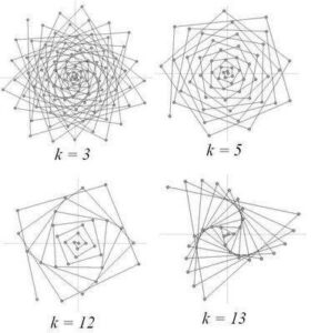
Because of how we have wound our  number spiral, quadratic sequences are particularly nice to plot. So how can we possibly resist spiral-plotting the 2-dimensional polygonal numbers? The plots below are of the 2-dimensional k-polygonal numbers for k = 3, 5, 12, and 13, that fall between 1 and 5000.

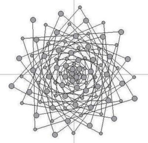
Plotting two polygonal number sequences on the same spiral gives us a way to see some of the numbers for which the sequences overlap (they do this at what are called highly polygonal numbers). For example, it turns out that every hexagonal number is also a triangular number. The image below shows an overlay of both the k = 6 and k = 3 sequences – numbers that are both hexagonal and triangular are shown as large dots, while the non-hexagonal triangular numbers are smaller.

The square and triangular number sequences line up less exactly than the hexagonal and triangular example above, but their overlap represents a well-known sequence in its own right (Sloane A001110 – see also wikipedia). The square-triangular sequence comes up surprisingly often in recreational mathematics, including a recently in an article about inquisitive computing by Brain Hayes. In the image below, the square numbers are squares, the triangular numbers are dots, and those that are both show up as triangles (1, 36, and  1225 are shown).

For more such insights, log into www.international-maths-challenge.com.

*Credit for article given to dan.mackinnon*

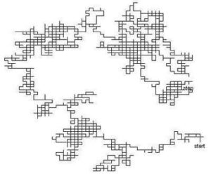
With connections to the study of gambling, Brownian motion, fractals, and more, random walks are a favourite topic in recreational mathematics.

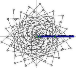
The diagram above (from Energy transformations during horizontal walking by F. G. Benedict and H. Murschhauser, published in 1915) suggests one method for generating walking data. Creating random walk simulations in Fathom or TinkerPlots is a little more straightforward.

First simulation – using sliders to determine a ‘base angle’

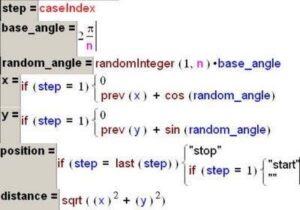
This first example lets you set up random walks where the direction chosen is based on an angle k*2pi/n for a fixed n (whose value is determined by a slider) and a random k (a random integer between 1 and n).

First, create a slider n, then create the attributes below and finally add the data (any number is fine – start with ~500 cases). The formulas below were entered in TinkerPlots, but would work equally well in Fathom.

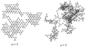
Plots of (x,y) will show the walk, and plots of (step, distance) will show how the distance from the origin changes over the course of the walk. Different values for n provide walks with their own particular geometries.

The walks start at (0,0) and wander about the plane from there. Re-randomizing (CNTRL-Y) generates new walks.

The simulation gives lots of nice pictures of random walks. You could generate statistics from these by adding measures and measure collections.

One limitation of this simulation is that it is difficult to determine exactly when the walker has returned to the start (0,0).  This turns out to be an interesting question for random walks on the plane (see the wikipedia entry for more on this). Because of the inexactness in the positions calculated using sine and cosine, the walker seems to never return to the origin. There are several ways of dealing with this, but one is to design a simpler simulation that uses exact values – one that sticks to lattice points (x, y), where x and y are both integers.

Second simulation – sticking to Integer lattice points

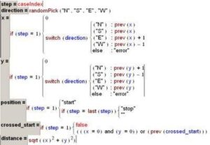
This second simulation can be thought of an ‘urban walker’ where all paths must follow a strictly laid out grid, like some downtown streets. The exactness of the positions means that we can detect with confidence when the walker has crossed back to their starting point. For this simulation, no slider is required – just enter the attributes and add cases.

Using the crossed_start attribute as a filter or to gather measures, you will find that walks often quickly pass over the starting point. You will also find that as you increase the number of cases, the straight ‘etch-a-sketch’ lines of the urban walk take on very interesting fractal-like contours.

For more such insights, log into www.international-maths-challenge.com.

*Credit for article given to dan.mackinnon*

 

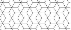
It could be argued that the square is the ‘nicest’ rhombus, but the rhombus with angles of 60 and 120 degrees seems nicer still. One of the nice things about the 60/120 rhomb are the plane tilings that can be constructed from it. One of these tilings is the ‘tumbling blocks’ tiling shown at the top of the post, in which at some points you see ‘cubes’ (around the degree 3 vertices), while at others you see ‘flowers’ (around the degree 6 vertices). Because of the two different types of vertices, this is known as a quasi-regular rhombic tiling. (Another tiling that uses the 60/120 rhomb is this one.)

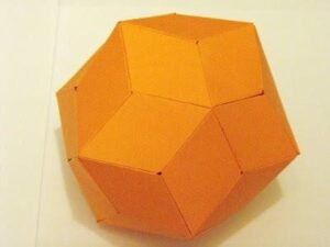
If you want to build a polyhedron that resembles the tumbling block tiling, one method is to reduce the number of petals in your flowers to 5, and then stretch your 60/120 rhombs until they are have angles of 63.435 and 116.565 degrees. Thirty of these rhombs arranged around vertices of degree 3 and 5 produces a quasi-regular polygon known as the rhombic triacontahedron.

The image above is of a model that was built using rhombic units printed onto card stock.

Despite the apparent ugliness of the 63.435 and 116.565 degree angle-measurements, our nice 60/120 rhomb has been, arguably, stretched into an even nicer one – a ‘golden rhombus,’ so called because the ratio of the diagonals is equal to the golden ratio.

The dual of the rhombic triacontahedron is the archemedian polyhedron known as the icosidodecahedron.

For more such insights, log into www.international-maths-challenge.com.

*Credit for article given to dan.mackinnon*

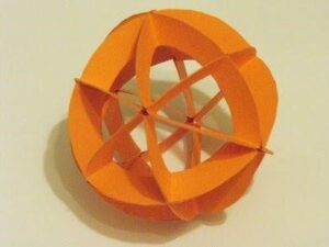
Imagine a tetrahedron centered inside a sphere. If you were to project the edges of the tetrahedron out from the center so that they touched the surface of the sphere, the edges would cut the sphere in arcs that lie on the sphere’s ‘great circles’ (the largest possible circles drawn on the surface of the sphere – circles whose radii are the same as the radius of the sphere).

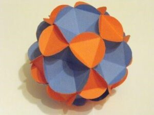
The image at the top of this post shows a model of a sphere with the six great circles formed by the projected edges of a tetrahedron sitting at its center.

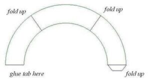
The model, described on pages 4 and 5 of Magnus Wennigers’ Polyhedron Models, is easy to construct using the template shown below. Printing copies of the template onto card-stock and gluing them together works well. This pdf file has 10 arcs on a single page for printing (you will need 24 arcs in total).

Each arc is folded and glued to form a spherical triangle, 24 of the spherical triangles glued together will form the sphere.

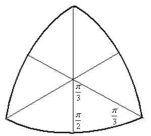
The diagram below (based on Fig.2, p.5, in Wenniger) shows how to assemble 6 of the triangles into one ‘face’ of the spherical tetrahedron. Four of the faces can be assembled into the ‘spherical tetrahedron.’ When assembling, you should make sure that you align the triangles so that they form great circles.

Spherical triangles, as you can tell from the diagram, do not follow the rule of having their interior angles sum to pi (180 degrees), as plane triangles do.

The arc is divided into angles of 54deg&44min, 70deg&32min, 54deg&44min, as described by Wenniger. The template was created in GSP.

For more such insights, log into www.international-maths-challenge.com.

*Credit for article given to dan.mackinnon*