Author: IMC

Both arithmetic aficionados and the mathematically challenged will be equally captivated by new research that upends hundreds of years of popular belief about prime numbers.

Contrary to what just about every mathematician on Earth will tell you, prime numbers can be predicted, according to researchers at City University of Hong Kong (CityUHK) and North Carolina State University, U.S.

The research team comprises Han-Lin Li, Shu-Cherng Fang, and Way Kuo. Fang is the Walter Clark Chair Professor of Industrial and Systems Engineering at North Carolina State University. Kuo is a Senior Fellow at the Hong Kong Institute for Advanced Study, CityU.

This is a genuinely revolutionary development in prime number theory, says Way Kuo, who is working on the project alongside researchers from the U.S. The team leader is Han-Lin Li, a Visiting Professor in the Department of Computer Science at CityUHK.

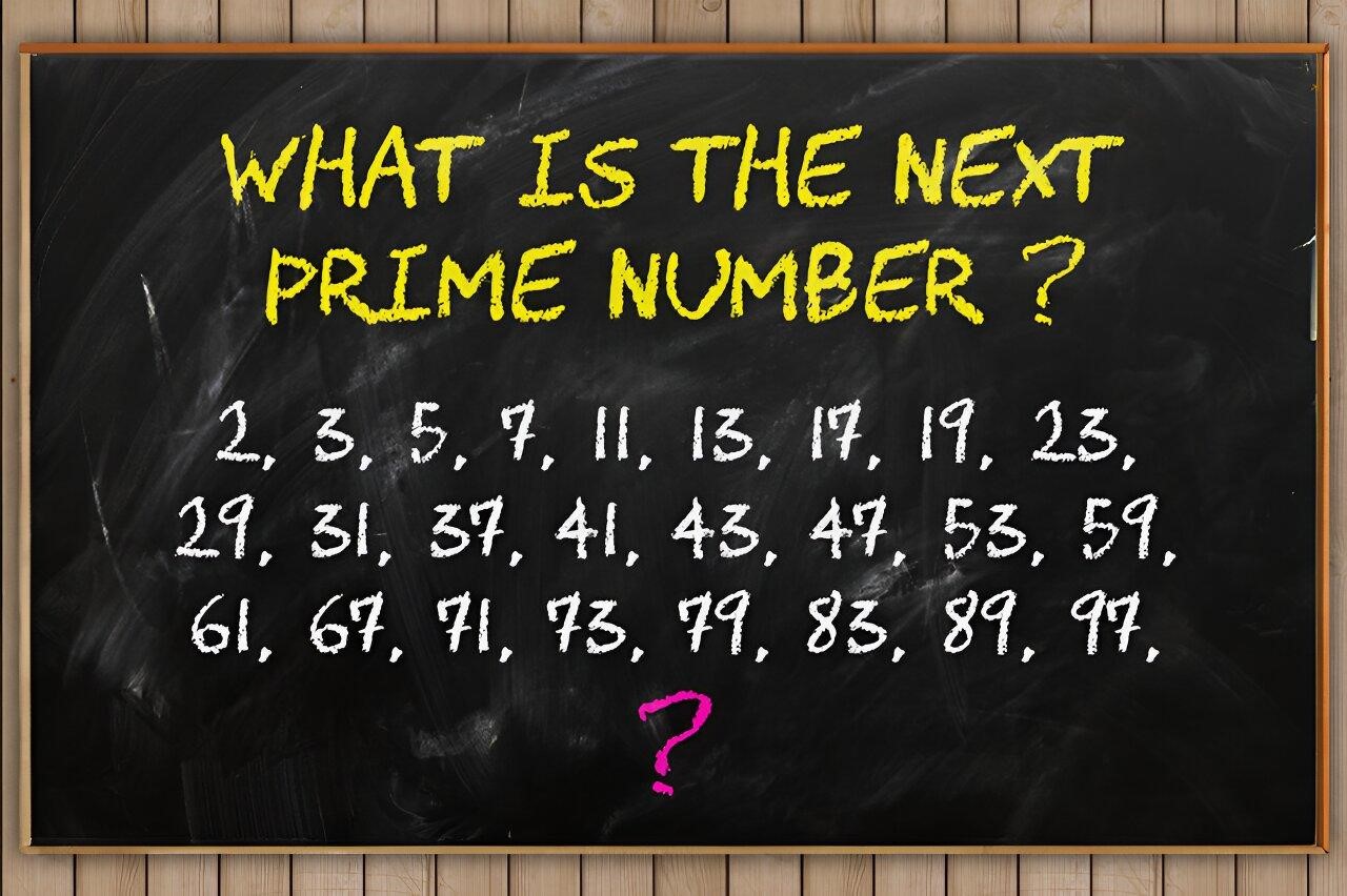
We have known for millennia that an infinite number of prime numbers, i.e., 2, 3, 5, 7, 11, etc., can be divided by themselves and the number 1 only. But until now, we have not been able to predict where the next prime will pop up in a sequence of numbers. In fact, mathematicians have generally agreed that prime numbers are like weeds: they seem just to shoot out randomly.

“But our team has devised a way to predict accurately and swiftly when prime numbers will appear,” adds Kuo.

The technical aspects of the research are daunting for all but a handful of mathematicians worldwide. In a nutshell, the outcome of the team’s research is a handy periodic table of primes, or the PTP, pointing the locations of prime numbers. The research is available as a working paper in the SSRN Electronic Journal.

The PTP can be used to shed light on finding a future prime, factoring an integer, visualizing an integer and its factors, identifying locations of twin primes, predicting the total number of primes and twin primes or estimating the maximum prime gap within an interval, among others.

More to the point, the PTP has major applications today in areas such as cyber security. Primes are already a fundamental part of encryption and cryptography, so this breakthrough means data can be made much more secure if we can predict prime numbers, Kuo explains.

This advance in prime number research stemmed from working on systems reliability design and a color coding system that uses prime numbers to enable efficient encoding and more effective color compression. During their research, the team discovered that their calculations could be used to predict prime numbers.

For more such insights, log into our website https://international-maths-challenge.com

Credit of the article given to Michael Gibb, City University of Hong Kong

Imagine if you enrolled your child in swimming lessons but instead of a qualified swimming instructor, they were taught freestyle technique by a soccer coach.

Something similar is happening in classrooms around Australia every day. As part of the ongoing teacher shortage, there are significant numbers of teachers teaching “out-of-field”. This means they are teaching subjects they are not qualified to teach.

One of the subjects where out-of-field teaching is particularly common is maths.

A 2021 report on Australia’s teaching workforce found that 40% of those teaching high school mathematics are out-of-field (English and science were 28% and 29%, respectively).

Another 2021 study of students in Year 8 found they were more likely to be taught by teachers who had specialist training in both maths and maths education if they went to a school in an affluent area rather than a disadvantaged one (54% compared with 31%).

Our new report looks at how we can fix this situation by training more existing teachers in maths education.

Why is this a problem?

Mathematics is one of the key parts of school education. But we are seeing worrying signs students are not receiving the maths education they need.

The 2021 study of Year 8 students showed those taught by teachers with a university degree majoring in maths had markedly higher results, compared with those taught by out-of-field teachers.

We also know maths skills are desperately needed in the broader workforce. The burgeoning worlds of big data and artificial intelligence rely on mathematical and statistical thinking, formulae and algorithms. Maths has also been identified as a national skill shortages priority area.

There are worrying signs students are not receiving the maths education they need. Aaron Lefler/ Unsplash, CC BY

What do we do about this?

There have been repeated efforts to address teacher shortages,including trying to retain existing mathematics teachers, having specialist teachers teaching across multiple schools and higher salaries. There is also a push to train more teachers from scratch, which of course will take many years to implement.

There is one strategy, however, that has not yet been given much attention by policy makers: upgrading current teachers’ maths and statistics knowledge and their skills in how to teach these subjects.

They already have training and expertise in how to teach and a commitment to the profession. Specific training in maths will mean they can move from being out-of-field to “in-field”.

How to give teachers this training

A new report commissioned by mathematics and statistics organisations in Australia (including the Australian Mathematical Sciences Institute) looks at what is currently available in Australia to train teachers in maths.

It identified 12 different courses to give existing teachers maths teaching skills. They varied in terms of location, duration (from six months to 18 months full-time) and aims.

For example, some were only targeted at teachers who want to teach maths in the junior and middle years of high school. Some taught university-level maths and others taught school-level maths. Some had government funding support; others could cost students more than A$37,000.

Overall, we found the current system is confusing for teachers to navigate. There are complex differences between states about what qualifies a teacher to be “in-field” for a subject area.

In the current incentive environment, we found these courses cater to a very small number of teachers. For example, in 2024 in New South Wales this year there are only about 50 government-sponsored places available.

This is not adequate. Pre-COVID, it was estimated we were losing more than 1,000 equivalent full-time maths teachers per year to attrition and retirement and new graduates were at best in the low hundreds.

But we don’t know exactly how many extra teachers need to be trained in maths. One of the key recommendations of the report is for accurate national data of every teacher’s content specialisations.

We need a national approach

The report also recommends a national strategy to train more existing teachers to be maths teachers. This would replace the current piecemeal approach.

It would involve a standard training regime across Australia with government and school-system incentives for people to take up extra training in maths.

There is international evidence to show a major upskilling program like this could work.

In Ireland, where the same problem was identified, the government funds a scheme run by a group of universities. Since 2012, teachers have been able to get a formal qualification (a professional diploma). Between 2009 and 2018 the percentage of out-of-field maths teaching in Ireland dropped from 48% to 25%.

To develop a similar scheme here in Australia, we would need coordination between federal and state governments and universities. Based on the Irish experience, it would also require several million dollars in funding.

But with students receiving crucial maths lessons every day by teachers who are not trained to teach maths, the need is urgent.

The report mentioned in this article was commissioned by the Australian Mathematical Sciences Institute, the Australian Mathematical Society, the Statistical Society of Australia, the Mathematics Education Research Group of Australasia and the Actuaries Institute.

For more such insights, log into our website https://international-maths-challenge.com

Credit of the article given to Monstera Production/ Pexels , CC BY

An attempt to settle a decade-long argument over a controversial proof by mathematician Shinichi Mochizuki has seen a war of words on both sides, with Mochizuki dubbing the latest effort as akin to a “hallucination” produced by ChatGPT,

An attempt to fix problems with a controversial mathematical proof has itself become mired in controversy, in the latest twist in a saga that has been running for over a decade and has seen mathematicians trading unusually pointed barbs.

The story began in 2012, when Shinichi Mochizuki at Kyoto University, Japan, published a 500-page proof of a problem called the ABC conjecture. The conjecture concerns prime numbers involved in solutions to the equation a + b = c, and despite its seemingly simple form, it provides deep insights into the nature of numbers. Mochizuki published a series of papers claiming to have proved ABC using new mathematical tools he collectively called Inter-universal Teichmüller (IUT) theory, but many mathematicians found the initial proof baffling and incomprehensible.

While a small number of mathematicians have since accepted that Mochizuki’s papers prove the conjecture, other researchers say there are holes in his argument and it needs further work, dividing the mathematical community in two and prompting a prize of up to $1 million for a resolution to the quandary.

Now, Kirti Joshi at the University of Arizona has published a proposed proof that he says fixes the problems with IUT and proves the ABC conjecture. But Mochizuki and his supporters, as well as mathematicians who critiqued Mochizuki’s original papers, remain unconvinced, with Mochizuki declaring that Joshi’s proposal doesn’t contain “any meaningful mathematical content whatsoever”.

Central to Joshi’s work is an apparent problem, previously identified by Peter Scholze at the University of Bonn, Germany, and Jakob Stix at Goethe University Frankfurt, Germany, with a part of Mochizuki’s proof called Conjecture 3.12. The conjecture involves comparing two mathematical objects, which Scholze and Stix say Mochizuki did incorrectly. Joshi claims to have found a more satisfactory way to make the comparison.

Joshi also says that his theory goes beyond Mochizuki’s and establishes a “new and radical way of thinking about arithmetic of number fields”. The paper, which hasn’t been peer-reviewed, is the culmination of several smaller papers on ABC that Joshi has published over several years, describing them as a “Rosetta Stone” for understanding Mochizuki’s impenetrable maths.

Neither Joshi nor Mochizuki responded to a request for comment on this article, and, indeed, the two seem reluctant to communicate directly with each other. In his paper, Joshi says Mochizuki hasn’t responded to his emails, calling the situation “truly unfortunate”. And yet, several days after the paper was posted online, Mochizuki published a 10-page response, saying that Joshi’s work was “mathematically meaningless” and that it reminded him of “hallucinations produced by artificial intelligence algorithms, such as ChatGPT”.

Mathematicians who support Mochizuki’s original proof express a similar sentiment. “There is nothing to talk about, since his [Joshi’s] proof is totally flawed,” says Ivan Fesenko at Westlake University in China. “He has no expertise in IUT whatsoever. No experts in IUT, and the number is in two digits, takes his preprints seriously,” he says. “It won’t pass peer review.”

And Mochizuki’s critics also disagree with Joshi. “Unfortunately, this paper and its predecessors does not introduce any powerful mathematical technology, and falls far short of giving a proof of ABC,” says Scholze, who has emailed Joshi to discuss the work further. For now, the saga continues.

For more such insights, log into www.international-maths-challenge.com.

*Credit for article given to Alex Wilkins*

This Easter season, as you tear open those chocolate eggs, have you ever wondered why they’re snugly wrapped in foil? Turns out the answer lies within the easter egg equation.

Mathematician Dr. Saul Schleimer, from the University of Warwick, sheds light on the delightful connection between Easter egg wrapping and mathematical curvature.

“When you wrap an egg with foil, there are always wrinkles in the foil. This doesn’t happen when you wrap a box. The reason is that foil has zero Gaussian curvature (a measure of flatness), while an egg has (variable) positive curvature. Perfect wrapping (without wrinkles) requires that the curvatures match,” explains Professor Schleimer.

So, unlike flat surfaces, eggs have variable positive curvature, making them challenging to wrap without creases or distortions. Foil, with its flat surface and zero Gaussian curvature, contrasts sharply with the egg’s curved shape.

Attempting to wrap an egg with paper, which also lacks the required curvature, would result in unsightly wrinkles and a less-than-ideal presentation. Therefore, by using tin foil, we can harmonize the egg’s curvature with the wrapping material, achieving a snug fit without compromising its shape, thus showcasing the delightful intersection of mathematics and Easter traditions.

For more such insights, log into our website https://international-maths-challenge.com

Credit of the article given to University of Warwick

For Michel Talagrand, who won the Abel mathematics prize on Wednesday, math provided a fun life free from all constraints—and an escape from the eye problems he suffered as a child.

“Math, the more you do it, the easier it gets,” the 72-year-old said in an interview with AFP.

He is the fifth French Abel winner since the award was created by Norway’s government in 2003 to compensate for the lack of a Nobel prize in mathematics.

Talagrand’s career in functional analysis and probability theorysaw him tame some of the incredibly complicated limits of random behaviour.

But the mathematician said he had just been “studying very simple things by understanding them absolutely thoroughly.”

Talagrand said he was stunned when told by the Norwegian Academy of Science and Letters that he had won the Abel prize.

“I did not react—I literally didn’t think for at least five seconds,” he said, adding that he was very happy for his wife and two children.

Fear of going blind

When he was young, Talagrand only turned to math “out of necessity,” he said.

By the age of 15, he had endured multiple retinal detachments and “lived in terror of going blind”.

Unable to run around with friends in Lyon, Talagrand immersed himself in his studies.

His father had a math degree and so he followed the same path. He said he was a “mediocre” student in other areas.

Talagrand was particularly poor at spelling, and still lashes out at what he calls its “arbitrary rules”.

Especially in comparison to math, which has “an order in which you do well if you are sensitive to it,” he said.

In 1974, Talagrand was recruited by the French National Centre for Scientific Research (CNRS), before getting a Ph.D. at Paris VI University.

He spent a decade studying functional analysis before finding his “thing”: probability.

It was then that Talagrand developed his influential theory about “Gaussian processes,” which made it possible to study some random phenomena.

Australian mathematician Matt Parker said that Talagrand had helped tame these “complicated random processes”.

Physicists had previously developed theories on the limits of how randomness behaves, but Talagrand was able to use mathematics to prove these limits, Parker said on the Abel Prize website.

‘Monstrously complicated’

“In a sense, things are as simple as could be—whereas mathematical objects can be monstrously complicated,” Talagrand said.

His work deepening the understanding of random phenomena “has become essential in today’s world,” the CNRS said, citing algorithms which are “the basis of our weather forecasts and our major linguistic models”.

Rather than creating a “brutal transformation”, Talagrand considers his discoveries as a collective work he compared to “the construction of a cathedral in which everyone lays a stone”.

He noted that French mathematics had been doing well an elite level, notching up both Abel prizes and Fields medals—the other equivalent to a math Nobel, which is only awarded to mathematicians under 40.

“But the situation is far less brilliant in schools,” where young people are increasingly less attracted to the discipline, he lamented.

The new Abel winner admitted that math can be daunting at first, but re-emphasized his belief that it gets easier the more you do it.

He advised aspiring mathematicians not to worry about failure.

“You can fail to solve a problem 10 times—but that doesn’t matter if you succeed on the 11th try,” he said.

It can also be hard work.

“All my life I worked to the point of exhaustion—but I had such fun!” he said.

“With math, you have all the resources within yourself. You work without any constraints, free from concerns about money or bosses,” he added.

“It’s marvelous.”

Talagrand will receive his prize, including a 7.5-million-kroner ($705,000) check, in Oslo on May 21.

For more such insights, log into our website https://international-maths-challenge.com

Credit of the article given to Juliette Collen

Chinese ice-ray lattice, or “binglie” as it is called in Chinese, is an intricate pattern that looks like cracked ice and is a common decorative element used in traditional Chinese window designs.

Originally inspired by fragmented patterns on ice or crackle-glazed ceramic surfaces, the design represents the melting of the ice and the beginning of a thriving spring.

When Dr. Iasef Md Rian, now an Associate Professor at Xi’an Jiaotong-Liverpool University’s Department of Architecture, arrived in China for the first time in 2019, he was immediately captivated by the latticed window designs in the classical gardens of Suzhou.

“Classical gardens in China strike me as very different from the Western ones, which are more symmetrical and organized,” he says. “Chinese gardens, however, have a more natural formation in their layout and design. The ice-ray window design is one of the manifestations.”

Having focused on fractal geometry in architectural design for many years, Dr. Rian felt an urge to explore the beauty in the patterns.

“My mind is always looking for this kind of inspiration source, so I was motivated right away to study the underlying geometric principles of the ice-ray patterns, he says.”

Revealing the underlying rule

Dr. Rian finds that the rule of creating ice-ray patterns is actually very simple.

He explains, “Take Type 1 as an example; a square is first divided into two quadrilaterals, and then each quadrilateral is further divided into two quadrilaterals. In each step, the proportions of the subdivided quadrilaterals are different, and this is how the random pattern is created using a simple rule.

“Through this configuration, Chinese craftsmen might have intended to increase its firmness so it can function as a window fence to provide protection. The random configuration of ice-ray lattices provides multi-angled connections, which transform the window into a collection of resultant forces and uniform stress distribution, in turn achieving a unique degree of stiffness.

“The microstructure of trabecular bone tissue in our own bodies serves as an excellent natural example of the potential of random lattices. It balances high stiffness, which contributes to strength, with a surprisingly lightweight structure.”

Dr. Rian recently published a paper in Frontiers of Architectural Research that explores the geometric qualities of ice-ray patterns and expands the possibilities of integrating random patterns into structural designs, especially the lattice shell design, which is often used in spherical domes and curved structures.

“In my research, I developed an algorithm to model the ice-ray patterns for lattice shell designs and assessed their feasibility and effectiveness compared to conventional gridshells. These gridshells, made from regular grids, contrast with continuous shells.

“While regular gridshells perform well under uniform loads, the ice-ray lattice offers strength under asymmetric loads. Some ice-ray patterns, resulting from optimization, surprisingly provide better strength than regular gridshells under self-weight. There is also an additional aesthetic advantage when applying the ice-ray pattern to a lattice shell design.

“I extend the application of this pattern to curved surfaces, which helps to unlock its potential in the geometric, structural, and constructional aspects of lattice shell design,” he says.

Dr. Rian has also integrated ice-ray patterns and complex geometries into his teaching. In 2022, he organized a workshop for students to design ice-ray lattice roofs.

He explains that learning the concept of fractal geometry can really push the students’ ideas toward a unique design.

“This is very different from what they’ve learned in high school. In learning to create this geometry system, they will also learn computational modeling and simulations. In the end, they’ll get comprehensive knowledge of advanced architectural and digital design,” he says.

Rediscovering traditional designs

To extend the research in this field, Dr. Rian is investigating the effectiveness of complex geometry in various aspects like micro-scale material design and structural design.

He says, “For instance, in facade design, we usually use conventional or parametric geometry to design regular shapes. However, the random shapes designed with complex geometry can offer a more natural impression and daylight penetration.”

He encourages design students and researchers to learn from the past.

“Any traditional design has a hidden rule in it. We can now use digital technologies and advanced tools to extend and expand the knowledge of traditional craftsmanship for contemporary design.

“There are many inspirations behind the traditional designs, and those principles can really inspire us designers to make innovative designs for the future,” he says.

For more such insights, log into our website https://international-maths-challenge.com

Credit of the article given to Yi Qian, Xi’an jiaotong-Liverpool University

There are no rabbits pulled out of hats here – these tricks rely on mathematical principles and will never fail you, says Peter Rowlett.

LOOK, I’ve got nothing up my sleeves. There are magic tricks that work by sleight of hand, relying on the skill of the performer and a little psychology. Then there are so-called self-working magic tricks, which are guaranteed to work by mathematical principles.

For example, say I ask you to write down a four-digit number and show me. I will write a prediction but keep it secret. Write another four-digit number and show me, then I will write one and show you. Now, sum the three visible numbers and you may be surprised to find the answer matches the prediction I made when I had only seen one number!

The trick is that while the number I wrote and showed you appeared random, I was actually choosing digits that make 9 when added to the digits of your second number. So if you wrote 3295, I would write 6704. This means the two numbers written after I made my prediction sum to 9999. So, my prediction was just your original number plus 9999. This is the same as adding 10,000 and subtracting 1, so I simply wrote a 1 to the left of your number and decreased the last digit by 1. If you wrote 2864, I would write 12863 as my prediction.

Another maths trick involves a series of cards with numbers on them (pictured). Someone thinks of a number and tells you which of the cards their number appears on. Quick as a flash, you tell them their number. You haven’t memorised anything; the trick works using binary numbers.

Regular numbers can be thought of as a series of columns containing digits, with each being 10 times the previous. So the right-most digit is the ones, to its left is the tens, then the hundreds, and so on. Binary numbers also use columns, but with each being worth two times the one to its right. So 01101 means zero sixteens, one eight, one four, zero twos and one one: 8+4+1=13.

Each card in this trick represents one of the columns in a binary number, moving from right to left: card 0 is the ones column, card 1 is the twos column, etc. Numbers appear on a card if their binary equivalent has a 1 in that place, and are omitted if it has a 0 there. For instance, the number 25 is 11001 in binary, so it is on cards 0, 3 and 4.

You can work this trick by taking the cards the person’s number appears on and converting them to their binary columns. From there, you can figure out the binary number and convert it to its regular number. But here’s a simple shortcut: the binary column represented by each card is the first number on the card, so you can just add the first number that appears on the cards the person names. So, for cards 0 and 2, you would add 1 and 4 to get 5.

Many self-working tricks embed mathematical principles in card magic, memorisation tricks or mind-reading displays, making the maths harder to spot. The key is they work every time.

For more such insights, log into www.international-maths-challenge.com.

*Credit for article given to Peter Rowlett*

After losing an eye at the age of 5, the 2024 Abel prize winner Michel Talagrand found comfort in mathematics.

French mathematician Michel Talagrand has won the 2024 Abel prize for his work on probability theory and describing randomness. Shortly after he had heard the news, New Scientist spoke with Talagrand to learn more about his mathematical journey.

Alex Wilkins: What does it mean to win the Abel prize?

Michel Talagrand: I think everybody would agree that the Abel prize is really considered like the equivalent of the Nobel prize in mathematics. So it’s something for me totally unexpected, I never, ever dreamed I would receive this prize. And actually, it’s not such an easy thing to do, because there is this list of people who already received it. And on that list, they are true giants of mathematics. And it’s not such a comfortable feeling to sit with them, let me tell you, because it’s clear that their achievements are on an entirely other scale than I am.

What are your attributes as a mathematician?

I’m not able to learn mathematics easily. I have to work. It takes a very long time and I have a terrible memory. I forget things. So I try to work, despite handicaps, and the way I worked was trying to understand really well the simple things. Really, really well, in complete detail. And that turned out to be a successful approach.

Why does maths appeal to you?

Once you are in mathematics, and you start to understand how it works, it’s completely fascinating and it’s very attractive. There are all kinds of levels, you are an explorer. First, you have to understand what people before you did, and that’s pretty challenging, and then you are on your own to explore, and soon you love it. Of course, it is extremely frustrating at the same time. So you have to have the personality that you will accept to be frustrated.

But my solution is when I’m frustrated with something, I put it aside, when it’s obvious that I’m not going to make any more progress, I put it aside and do something else, and I come back to it at a later date, and I have used that strategy with great efficiency. And the reason why it succeeds is the function of the human brain, things mature when you don’t look at them. There are questions which I’ve literally worked on for a period of 30 years, you know, coming back to them. And actually at the end of the 30 years, I still made progress. That’s what is incredible.

How did you get your start?

Now, that’s a very personal story. First, it helps that my father was a maths teacher, and of course that helped. But really, the determining factor is I was unlucky to have been born with a deficiency in my retinas. And I lost my right eye when I was 5 years old. I had multiple retinal detachments when I was 15. I stayed in the hospital a long time, I missed school for six months. And that was extremely traumatic, I lived in constant terror that there will be a next retinal detachment.

To escape that, I started to study. And my father really immensely helped me, you know, when he knew how hard it was, and when I was in hospital, he came to see me every day and he started talking about some simple mathematics, just to keep my brain functioning. I started studying hard mathematics and physics to really, as I say, to fight the terror and, of course, when you start studying, then you become good at it and once you become good, it’s very appealing.

What is it like to be a professional mathematician?

Nobody tells me what I have to do and I’m completely free to use my time and do what I like. That fitted my personality well, of course, and it’s helped me to devote myself totally to my work.

For more such insights, log into www.international-maths-challenge.com.

*Credit for article given to Alex Wilkins*

Fermat’s last theorem puzzled mathematicians for centuries until it was finally proven in 1993. Now, researchers want to create a version of the proof that can be formally checked by a computer for any errors in logic.

Mathematicians hope to develop a computerised proof of Fermat’s last theorem, an infamous statement about numbers that has beguiled them for centuries, in an ambitious, multi-year project that aims to demonstrate the potential of computer-assisted mathematical proofs.

Pierre de Fermat’s theorem, which he first proposed around 1640, states that there are no integers, or whole numbers, a, b, and c that satisfy the equation aⁿ + bⁿ = cⁿ for any integer n greater than 2. Fermat scribbled the claim in a book, famously writing: “I have discovered a truly marvellous proof of this, which this margin is too narrow to contain.”

It wasn’t until 1993 that Andrew Wiles, then at Princeton University, set the mathematical world alight by announcing he had a proof. Spanning more than 100 pages, the proof contained such advanced mathematics that it took more than two years for his colleagues to verify it didn’t contain any errors.

Many mathematicians hope that this work of checking, and eventually writing, proofs can be sped up by translating them into a computer-readable language. This process of formalisation would let computers instantly spot logical mistakes and, potentially, use the theorems as building blocks for other proofs.

But formalising modern proofs can itself be tricky and time-consuming, as much of the modern maths they rely on is yet to be made machine-readable. For this reason, formalising Fermat’s last theorem has long been considered far out of reach. “It was regarded as a tremendously ambitious proof just to prove it in the first place,” says Lawrence Paulson at the University of Cambridge.

Now, Kevin Buzzard at Imperial College London and his colleagues have announced plans to take on the challenge, attempting to formalise Fermat’s last theorem in a programming language called Lean.

“There’s no point in Fermat’s last theorem, it’s completely pointless. It doesn’t have any applications – either theoretical or practical – in the real world,” says Buzzard. “But it’s also a really hard question that’s become infamous because, for centuries, people have generated loads of brilliant new ideas in an attempt to solve it.”

He hopes that by formalising many of these ideas, which now include routine mathematical tools in number theory such as modular forms and Galois representations, it will help other researchers whose work is currently too far beyond the scope of computer assistants.

“It’s the kind of project that could have quite far-reaching and unexpected benefits and consequences,” says Chris Williams at the University of Nottingham, UK.

The proof itself will loosely follow Wiles’s, with slight modifications. A publicly available blueprint will be available online once the project is live, in April, so that anyone from Lean’s fast-growing community can contribute to formalising sections of the proof.

“Ten years ago, this would have taken an infinite amount of time,” says Buzzard. Even so, he will be concentrating on the project full-time from October, putting his teaching responsibilities on hold for five years in an effort to complete it.

“I think it’s unlikely he’ll be able to formalise the entire proof in the next five years, that would be a staggering achievement,” says Williams. “But because a lot of the tools that go into it are so ubiquitous now in number theory and arithmetic geometry, I’d expect any substantial progress towards it would be very useful in the future.”

For more such insights, log into www.international-maths-challenge.com.

*Credit for article given to Alex Wilkins*

Math enthusiasts around the world, from college kids to rocket scientists, celebrate Pi Day on Thursday, which is March 14 or 3/14—the first three digits of an infinite number with many practical uses.

Around the world many people will mark the day with a slice of pie—sweet, savory or even pizza.

Simply put, pi is a mathematical constant that expresses the ratio of a circle’s circumference to its diameter. It is part of many formulas used in physics, astronomy, engineering and other fields, dating back thousands of years to ancient Egypt, Babylon and China.

Pi Day itself dates to 1988, when physicist Larry Shaw began celebrations at the Exploratorium science museum in San Francisco. The holiday didn’t really gain national recognition though until two decades later. In 2009, Congress designated every March 14 to be the big day—to hopefully spur more interest in math and science. Fittingly enough, the day is also Albert Einstein’s birthday.

Here’s a little more about the holiday’s origin and how it’s celebrated today.

WHAT IS PI?

Pi can calculate the circumference of a circle by measuring the diameter—the distance straight across the circle’s middle—and multiplying that by the 3.14-plus number.

It is considered a constant number and it is also infinite, meaning it is mathematically irrational. Long before computers, historic scientists such as Isaac Newton spent many hours calculating decimal places by hand. Today, using sophisticated computers, researchers have come up with trillions of digits for pi, but there is no end.

WHY IS IT CALLED PI?

It wasn’t given its name until 1706, when Welsh mathematician William Jones began using the Greek symbol for the number.

Why that letter? It’s the first Greek letter in the words “periphery” and “perimeter,” and pi is the ratio of a circle’s periphery—or circumference—to its diameter.

WHAT ARE SOME PRACTICAL USES?

The number is key to accurately pointing an antenna toward a satellite. It helps figure out everything from the size of a massive cylinder needed in refinery equipment to the size of paper rolls used in printers.

Pi is also useful in determining the necessary scale of a tank that serves heating and air conditioning systems in buildings of various sizes.

NASA uses pi on a daily basis. It’s key to calculating orbits, the positions of planets and other celestial bodies, elements of rocket propulsion, spacecraft communication and even the correct deployment of parachutes when a vehicle splashes down on Earth or lands on Mars.

Using just nine digits of pi, scientists say it can calculate the Earth’s circumference so accurately it only errs by about a quarter of an inch (0.6 centimeters) for every 25,000 miles (about 40,000 kilometers).

IT’S NOT JUST MATH, THOUGH

Every year the San Francisco museum that coined the holiday organizes events, including a parade around a circular plaque, called the Pi Shrine, 3.14 times—and then, of course, festivities with lots of pie.

Around the country, many events now take place on college campuses. For example, Nova Southeastern University in Florida will hold a series of activities, including a game called “Mental Math Bingo” and event with free pizza (pies)—and for dessert, the requisite pie.

“Every year Pi Day provides us with a way to celebrate math, have some fun and recognize how important math is in all our lives,” said Jason Gershman, chair of NSU’s math department.

At Michele’s Pies in Norwalk, Connecticut, manager Stephen Jarrett said it’s one of their biggest days of the year.

“We have hundreds of pies going out for orders (Thursday) to companies, schools and just individuals,” Jarrett said in an interview. “Pi Day is such a fun, silly holiday because it’s a mathematical number that people love to turn into something fun and something delicious. So people celebrate Pi Day with sweet pies, savory pies, and it’s just an excuse for a little treat.”

NASA has its annual “Pi Day Challenge” online, offering people plenty of games and puzzles, some of them directly from the space agency’s own playbook such as calculating the orbit of an asteroid or the distance a moon rover would need to travel each day to survey a certain lunar area.

WHAT ABOUT EINSTEIN?

Possibly the world’s best-known scientist, Einstein was born on March 14, 1879, in Germany. The infinite number of pi was used in many of his breakthrough theories and now Pi Day gives the world another reason to celebrate his achievements.

In a bit of math symmetry, famed physicist Stephen Hawking died on March 14, 2018, at age 76. Still, pi is not a perfect number. He once had this to say,

“One of the basic rules of the universe is that nothing is perfect. Perfection simply doesn’t exist. Without imperfection, neither you nor I would exist.”

For more such insights, log into our website https://international-maths-challenge.com

Credit of the article given to Curt Anderson