A pair of mathematicians studied the UK National Lottery and figured out a combination of 27 tickets that guarantees you will always win, but they tell New Scientist they don’t bother to play.
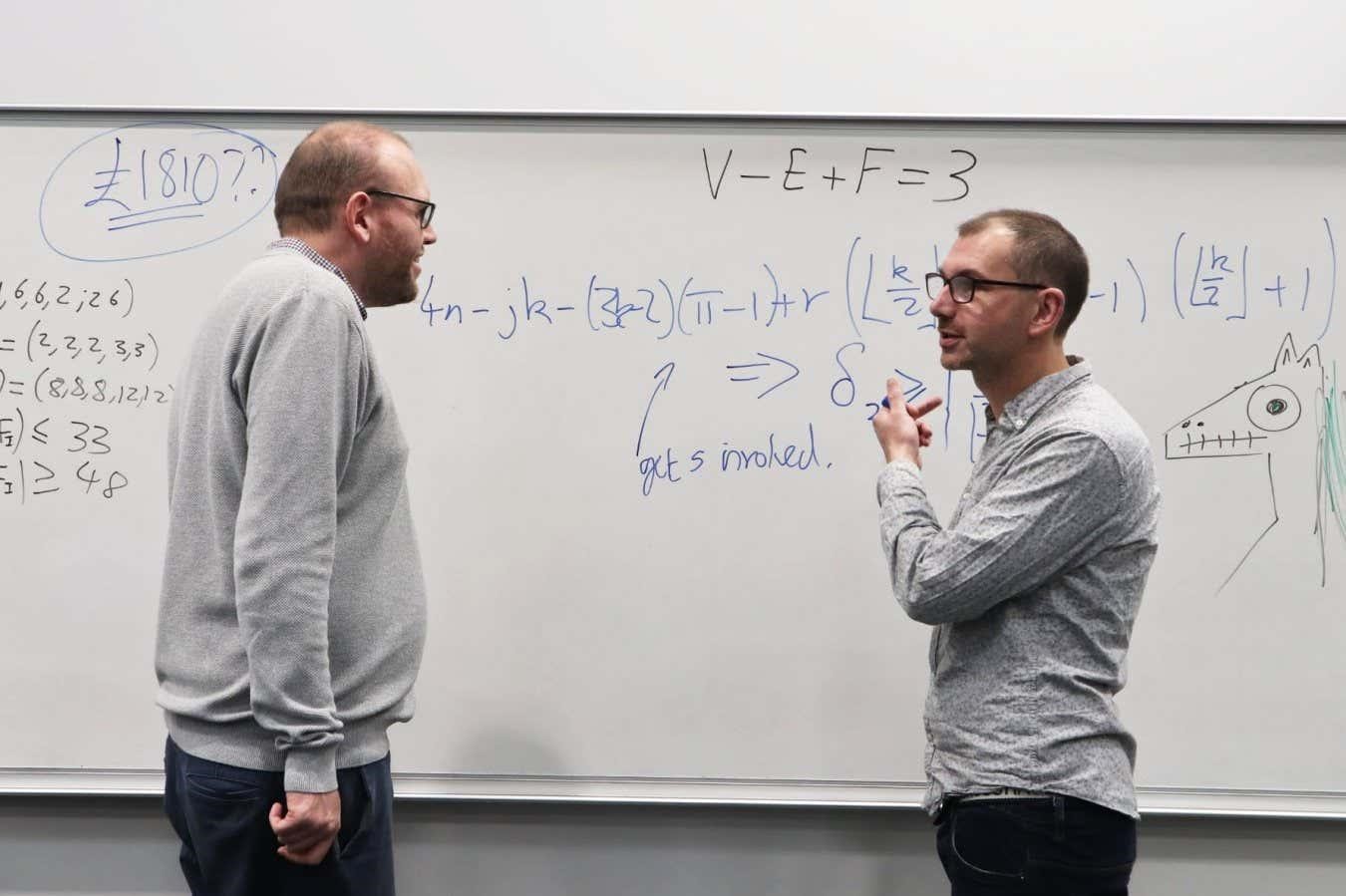
David Cushing and David Stewart calculate a winning solution
Earlier this year, two mathematicians revealed that it is possible to guarantee a win on the UK national lottery by buying just 27 tickets, despite there being 45,057,474 possible draw combinations. The pair were shocked to see their findings make headlines around the world and inspire numerous people to play these 27 tickets – with mixed results – and say they don’t bother to play themselves.
David Cushing and David Stewart at the University of Manchester, UK, used a mathematical field called finite geometry to prove that particular sets of 27 tickets would guarantee a win.
They placed each of the lottery numbers from 1 to 59 in pairs or triplets on a point within one of five geometrical shapes, then used these to generate lottery tickets based on the lines within the shapes. The five shapes offer 27 such lines, meaning that 27 tickets will cover every possible winning combination of two numbers, the minimum needed to win a prize. Each ticket costs £2.
It was an elegant and intuitive solution to a tricky problem, but also an irresistible headline that attracted newspapers, radio stations and television channels from around the world. And it also led many people to chance their luck – despite the researchers always pointing out that it was, statistically speaking, a very good way to lose money, as the winnings were in no way guaranteed to even cover the cost of the tickets.
Cushing says he has received numerous emails since the paper was released from people who cheerily announce that they have won tiny amounts, like two free lucky dips – essentially another free go on the lottery. “They were very happy to tell me how much they’d lost basically,” he says.
The pair did calculate that their method would have won them £1810 if they had played on one night during the writing of their research paper – 21 June. Both Cushing and Stewart had decided not to play the numbers themselves that night, but they have since found that a member of their research group “went rogue” and bought the right tickets – putting himself £1756 in profit.
“He said what convinced him to definitely put them on was that it was summer solstice. He said he had this feeling,” says Cushing, shaking his head as he speaks. “He’s a professional statistician. He is incredibly lucky with it; he claims he once found a lottery ticket in the street and it won £10.”
Cushing and Stewart say that while their winning colleague – who would prefer to remain nameless – has not even bought them lunch as a thank you for their efforts, he has continued to play the 27 lottery tickets. However, he now randomly permutes the tickets to alternative 27-ticket, guaranteed-win sets in case others have also been inspired by the set that was made public. Avoiding that set could avert a situation where a future jackpot win would be shared with dozens or even hundreds of mathematically-inclined players.
Stewart says there is no way to know how many people are doing the same because Camelot, which runs the lottery, doesn’t release that information. “If the jackpot comes up and it happens to match exactly one of the [set of] tickets and it gets split a thousand ways, that will be some indication,” he says.
Nonetheless, Cushing says that he no longer has any interest in playing the 27 tickets. “I came to the conclusion that whenever we were involved, they didn’t make any money, and then they made money when we decided not to put them on. That’s not very mathematical, but it seemed to be what was happening,” he says.
And Stewart is keen to stress that mathematics, no matter how neat a proof, can never make the UK lottery a wise investment. “If every single man, woman and child in the UK bought a separate ticket, we’d only have a quarter chance of someone winning the jackpot,” he says.
For more such insights, log into www.international-maths-challenge.com.
*Credit for article given to Matthew Sparkes*