Category: Skills and Learning

Maths tells us the best way to cover a surface with copies of a shape – even when it comes to jigsaw puzzles, says Katie Steckles.

WHAT do a bathroom wall, a honeycomb and a jigsaw puzzle have in common? Obviously, the answer is mathematics.

If you are trying to cover a surface with copies of a shape – say, for example, you are tiling a bathroom – you ideally want a shape like a square or rectangle. They will cover the whole surface with no gaps, which is why these boring shapes get used as wall tiles so often.

But if your shapes don’t fit together exactly, you can still try to get the best coverage possible by arranging them in an efficient way.

Imagine trying to cover a surface with circular coins. The roundness of the circles means there will be gaps between them. For example, we could use a square grid, placing the coins on the intersections. This will cover about 78.5 per cent of the area.

But this isn’t the most efficient way: in 1773, mathematician Joseph-Louis Lagrange showed that the optimal arrangement of circles involves a hexagonal grid, like the cells in a regular honeycomb – neat rows where each circle sits nestled between the two below it.

In this situation, the circles will cover around 90.7 per cent of the space, which is the best you can achieve with this shape. If you ever need to cover a surface with same-size circles, or pack identical round things into a tray, the hexagon arrangement is the way to go.

But this isn’t just useful knowledge if you are a bee: a recent research paper used this hexagonal arrangement to figure out the optimal size table for working a jigsaw puzzle. The researchers calculated how much space would be needed to lay out the pieces of an unsolved jigsaw puzzle, relative to the solved version. Puzzle pieces aren’t circular, but they can be in any orientation and the tabs sticking out stop them from moving closer together, so each takes up a theoretically circular space on the table.

By comparing the size of the central rectangular section of the jigsaw piece to the area it would take up in the hexagonal arrangement, the paper concluded that an unsolved puzzle takes up around 1.73 times as much space.

This is the square root of three (√3), a number with close connections to the regular hexagon – one with a side length of 1 will have a height of √3. Consequently, there is also a √3 in the formula for the hexagon’s area, which is 3/2 × √3 × s², where s is the length of a side. This is partly why it pops out, after some fortuitous cancellation, as the answer here.

So if you know the dimensions of a completed jigsaw puzzle, you can figure out what size table you need to lay out all the pieces: multiply the width and height, then multiply that by 1.73. For this ingenious insight, we can thank the bees.

For more such insights, log into www.international-maths-challenge.com.

*Credit for article given to Katie Steckles*

School mathematics teaching is stuck in the past. An adult revisiting the school that they attended as a child would see only superficial changes from what they experienced themselves.

Yes, in some schools they might see a room full of electronic tablets, or the teacher using a touch-sensitive, interactive whiteboard. But if we zoom in on the details – the tasks that students are actually being given to help them make sense of the subject – things have hardly changed at all.

We’ve learnt a huge amount in recent years about cognitive science – how our brains work and how people learn most effectively. This understanding has the potential to revolutionise what teachers do in classrooms. But the design of mathematics teaching materials, such as textbooks, has benefited very little from this knowledge.

Some of this knowledge is counter-intuitive, and therefore unlikely to be applied unless done so deliberately. What learners prefer to experience, and what teachers think is likely to be most effective, often isn’t what will help the most.

For example, cognitive science tells us that practising similar kinds of tasks all together generally leads to less effective learning than mixing up tasks that require different approaches.

In mathematics, practising similar tasks together could be a page of questions each of which requires addition of fractions. Mixing things up might involve bringing together fractions, probability and equations in immediate succession.

Learners make more mistakes when doing mixed exercises, and are likely to feel frustrated by this. Grouping similar tasks together is therefore likely to be much easier for the teacher to manage. But the mixed exercises give the learner important practice at deciding what method they need to use for each question. This means that more knowledge is retained afterwards, making this what is known as a “desirable difficulty”.

Cognitive science applied

We are just now beginning to apply findings like this from cognitive science to design better teaching materials and to support teachers in using them. Focusing on school mathematics makes sense because mathematics is a compulsory subject which many people find difficult to learn.

Typically, school teaching materials are chosen by gut reactions. A head of department looks at a new textbook scheme and, based on their experience, chooses whatever seems best to them. What else can they be expected to do? But even the best materials on offer are generally not designed with cognitive science principles such as “desirable difficulties” in mind.

My colleagues and I have been researching educational designthat applies principles from cognitive science to mathematics teaching, and are developing materials for schools. These materials are not designed to look easy, but to include “desirable difficulties”.

They are not divided up into individual lessons, because this pushes the teacher towards moving on when the clock says so, regardless of student needs. Being responsive to students’ developing understanding and difficulties requires materials designed according to the size of the ideas, rather than what will fit conveniently onto a double-page spread of a textbook or into a 40-minute class period.

Switching things up

Taking an approach led by cognitive science also means changing how mathematical concepts are explained. For instance, diagrams have always been a prominent feature of mathematics teaching, but often they are used haphazardly, based on the teacher’s personal preference. In textbooks they are highly restricted, due to space constraints.

Often, similar-looking diagrams are used in different topics and for very different purposes, leading to confusion. For example, three circles connected as shown below can indicate partitioning into a sum (the “part-whole model”) or a product of prime factors.

These involve two very different operations, but are frequently represented by the same diagram. Using the same kind of diagram to represent conflicting operations (addition and multiplication) leads to learners muddling them up and becoming confused.

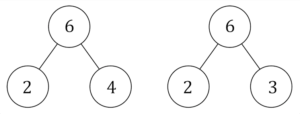
Number diagrams showing numbers that add together to make six and numbers that multiply to make six. Colin Foster

The “coherence principle” from cognitive science means avoiding diagrams where their drawbacks outweigh their benefits, and using diagrams and animations in a purposeful, consistent way across topics.

For example, number lines can be introduced at a young age and incorporated across many topic areas to bring coherence to students’ developing understanding of number. Number lines can be used to solve equations and also to represent probabilities, for instance.

Unlike with the circle diagrams above, the uses of number lines shown below don’t conflict but reinforce each other. In each case, positions on the number line represent numbers, from zero on the left, increasing to the right.

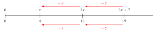
A number line used to solve an equation. Colin Foster

A number line used to show probability. Colin Foster

There are disturbing inequalities in the learning of mathematics, with students from poorer backgrounds underachieving relative to their wealthier peers. There is also a huge gender participation gap in maths, at A-level and beyond, which is taken by far more boys than girls.

Socio-economically advantaged families have always been able to buy their children out of difficulties by using private tutors, but less privileged families cannot. Better-quality teaching materials, based on insights from cognitive science, mitigate the impact for students who have traditionally been disadvantaged by gender, race or financial background in the learning of mathematics.

For more such insights, log into our website https://international-maths-challenge.com

Credit of the article given to SrideeStudio/Shutterstock

When choosing the perfectly sized table to do your jigsaw puzzle on, work out the area of the completed puzzle and multiply it by 1.73.

People may require a larger table if they like to lay all the pieces out at the start, rather than keeping them in the box or in piles

How large does your table need to be when doing a jigsaw puzzle? The answer is the area of the puzzle when assembled multiplied by 1.73. This creates just enough space for all the pieces to be laid flat without any overlap.

“My husband and I were doing a jigsaw puzzle one day and I just wondered if you could estimate the area that the pieces take up before you put the puzzle together,” says Madeleine Bonsma-Fisher at the University of Toronto in Canada.

To uncover this, Bonsma-Fisher and her husband Kent Bonsma-Fisher, at the National Research Council Canada, turned to mathematics.

Puzzle pieces take on a range of “funky shapes” that are often a bit rectangular or square, says Madeleine Bonsma-Fisher. To get around the variation in shapes, the pair worked on the basis that all the pieces took up the surface area of a square. They then imagined each square sitting inside a circle that touches its corners.

By considering the area around each puzzle piece as a circle, a shape that can be packed in multiple ways, they found that a hexagonal lattice, similar to honeycomb, would mean the pieces could interlock with no overlap. Within each hexagon is one full circle and parts of six circles.

They then found that the area taken up by the unassembled puzzle pieces arranged in the hexagonal pattern would always be the total area of the completed puzzle – calculated by multiplying its length by its width – multiplied by the root of 3, or 1.73.

This also applies to jigsaw puzzle pieces with rectangular shapes, seeing as these would similarly fit within a circle.

While doing a puzzle, some people keep pieces that haven’t yet been used in the box, while others arrange them in piles or lay them on a surface, the latter being Madeleine Bonsma-Fisher’s preferred method. “If you really want to lay all your pieces out flat and be comfortable, your table should be a little over twice as big as your sample puzzle,” she says.

For more such insights, log into www.international-maths-challenge.com.

*Credit for article given to Chen Ly*

A pair of mathematicians studied the UK National Lottery and figured out a combination of 27 tickets that guarantees you will always win, but they tell New Scientist they don’t bother to play.

David Cushing and David Stewart calculate a winning solution

Earlier this year, two mathematicians revealed that it is possible to guarantee a win on the UK national lottery by buying just 27 tickets, despite there being 45,057,474 possible draw combinations. The pair were shocked to see their findings make headlines around the world and inspire numerous people to play these 27 tickets – with mixed results – and say they don’t bother to play themselves.

David Cushing and David Stewart at the University of Manchester, UK, used a mathematical field called finite geometry to prove that particular sets of 27 tickets would guarantee a win.

They placed each of the lottery numbers from 1 to 59 in pairs or triplets on a point within one of five geometrical shapes, then used these to generate lottery tickets based on the lines within the shapes. The five shapes offer 27 such lines, meaning that 27 tickets will cover every possible winning combination of two numbers, the minimum needed to win a prize. Each ticket costs £2.

It was an elegant and intuitive solution to a tricky problem, but also an irresistible headline that attracted newspapers, radio stations and television channels from around the world. And it also led many people to chance their luck – despite the researchers always pointing out that it was, statistically speaking, a very good way to lose money, as the winnings were in no way guaranteed to even cover the cost of the tickets.

Cushing says he has received numerous emails since the paper was released from people who cheerily announce that they have won tiny amounts, like two free lucky dips – essentially another free go on the lottery. “They were very happy to tell me how much they’d lost basically,” he says.

The pair did calculate that their method would have won them £1810 if they had played on one night during the writing of their research paper – 21 June. Both Cushing and Stewart had decided not to play the numbers themselves that night, but they have since found that a member of their research group “went rogue” and bought the right tickets – putting himself £1756 in profit.

“He said what convinced him to definitely put them on was that it was summer solstice. He said he had this feeling,” says Cushing, shaking his head as he speaks. “He’s a professional statistician. He is incredibly lucky with it; he claims he once found a lottery ticket in the street and it won £10.”

Cushing and Stewart say that while their winning colleague – who would prefer to remain nameless – has not even bought them lunch as a thank you for their efforts, he has continued to play the 27 lottery tickets. However, he now randomly permutes the tickets to alternative 27-ticket, guaranteed-win sets in case others have also been inspired by the set that was made public. Avoiding that set could avert a situation where a future jackpot win would be shared with dozens or even hundreds of mathematically-inclined players.

Stewart says there is no way to know how many people are doing the same because Camelot, which runs the lottery, doesn’t release that information. “If the jackpot comes up and it happens to match exactly one of the [set of] tickets and it gets split a thousand ways, that will be some indication,” he says.

Nonetheless, Cushing says that he no longer has any interest in playing the 27 tickets. “I came to the conclusion that whenever we were involved, they didn’t make any money, and then they made money when we decided not to put them on. That’s not very mathematical, but it seemed to be what was happening,” he says.

And Stewart is keen to stress that mathematics, no matter how neat a proof, can never make the UK lottery a wise investment. “If every single man, woman and child in the UK bought a separate ticket, we’d only have a quarter chance of someone winning the jackpot,” he says.

For more such insights, log into www.international-maths-challenge.com.

*Credit for article given to Matthew Sparkes*

What is a Flipped Classroom?

Most teachers understand the “Chalk and Talk” or “Direct Instruction” method. The teacher begins by reviving what they did the day before, then continue with some new theories and concepts on the board, generally seeking student attention to work through the instances. Then once the maths students have the right set of notes from the board, they would use their textbook for a particular chapter, start solving the questions given by the teacher, and expectantly complete those tasks at home for homework.

As maths tutors, we are familiar that daily practice is significant. However, the students experience problems when practising, and their teacher isn’t there to assist them. The flipped classroom vision reorganizes what comes about at home and school compared to a more conventional plan. In short, the students will first find new content mainly independently, often as homework. Then in class, most of the time burnt out practising, finishing exercises, asking questions, and working on other activities in groups, with the teacher there to guide them.

Why do a Flipped Classroom?

Flipped classrooms permit one-on-one sessions with maths students who are practising, especially for the International Maths Olympiad, so we can move further in more effective directions. Change is challenging, so why do a flipped classroom? In short, change can be strenuous but productive. Bloom’s Two Sigma Problem demonstrates that a one-on-one session is the best method for teaching and learning.

How to Flip Maths Classroom?

Choose a topic to begin with, based on the timing, but you may select a topic that you believe matches the new strategy perfectly.

No matter your standard or plan for the organization, we suggest making a calendar to organize your unit before you begin.

It would be best if you had a simple outline of what lessons or concepts you will cover each day.

If you plan to create your own video sessions, you must figure out the best video recording practices.

Explain to students

If students are used to a specific teaching style and method, changing the pattern can also be an issue for them. It’s necessary to be clear with them about the switch that is taking place, why they’re happening, and what the students should anticipate in the outcome.

This is how one can flip for a maths classroom. Happy teaching!

You ordered a pizza for your party, but the restaurant forgot to slice it – these mathematical tricks can help you cut it evenly, says Katie Steckles.

Fairness is important – in life, and in pizza. If you want to cut a pizza into equal-sized pieces, the difficulty will depend on how many people you need to share it between. Luckily, mathematics has some tricks to keep things equal.

For example, if the number of people you are sharing a pizza between is a power of two – one, two, four, eight, 16 – cutting the pizza into as many slices is easy. For one piece, obviously no cuts are needed. For each larger power of two, a cut across through the centre of the pizza – cutting all of the existing pieces exactly in half – will result in pieces of equal size.

Some numbers will be much harder: prime numbers, by definition, can’t be divided easily. Luckily, geometry can help.

If you need to cut a pizza into five equal pieces, first grab a long, thin, rectangular strip of paper. Tie the paper in an ordinary overhand knot, like you would tie in a piece of string. Then, keeping the ends flat, pull gently to tighten the knot. The whole thing will flatten and come together – stop pulling when you can’t go any further without it wrinkling.

The flat shape you are looking at should now be vaguely familiar, if you ignore the two ends of paper sticking out. Fold these ends into the middle, or cut them off, and you will have a shape with five straight edges, created purely by the shape of the knot. Yes, that is right – you have made a perfect regular pentagon, with five equal-length sides and five equal angles at the corners.

It is possible to prove this mathematically by showing that all the folds you make in the paper strip are at 72 degrees to the parallel edges of the strip. But for simplicity, because the paper is the same width everywhere, and weaves in and out five times in the right way, these will be five equal edges. And more importantly, the pentagon’s corners are equally spread around a circle – making it the perfect guide for pizza slicing.

Place your pentagon in the centre of the pizza, then cut along lines radiating out from the centre of the pentagon and through each corner. And presto: you have a pentagonal pizza party for five. This paper-strip method can be used whenever you are in a pentagon-based emergency.

You can use the same technique to produce a shape with any odd number of sides by creating a more complex knot with the strip passing through the middle more times, although the strip of paper needs to be increasingly thin and it takes a lot more patience to pull the ends through and carefully flatten out the shape.

Combined with our existing halving methods, you can now produce any number of slices you like. The same results can be extended to any other round food – thanks to maths, the world is your cheesecake.

For more such insights, log into www.international-maths-challenge.com.

*Credit for article given to Katie Steckles *

Mathematics and engineering go hand in hand. Mathematics is an essential tool for engineers and plays a crucial role in helping students become better engineers. In this article, we will explore how math helps students become better engineers.

Understanding and Applying Principles:

Engineering is all about applying scientific principles to solve real-world problems. Mathematics is the language of science, and without it, engineers would not be able to understand the fundamental principles that govern the world around us. By studying math, students learn how to analyze and solve complex problems, which is a critical skill for any engineer. Moreover, math helps students understand the fundamental concepts of physics, which is essential to many engineering fields.

Analyzing and Solving Problems:

Engineers are problem solvers, and math is an essential tool for problem-solving. Math helps students develop critical thinking skills and teaches them how to analyze and solve problems systematically. Engineers use mathematical concepts to create models, analyze data, and make predictions. These models and predictions help engineers design and build products that meet specific needs and requirements. One standard approach to building your maths skills is by participating in Olympiads such as the International Maths Olympiad Challenge.

Design and Optimization:

Designing and optimizing systems is another essential part of engineering. Math plays a critical role in helping engineers design and optimize systems. Mathematical models help engineers simulate and optimize systems to ensure that they meet specific requirements. By understanding mathematical concepts like calculus, optimization, and linear algebra, students can learn how to design and optimize complex systems.

Communication:

Engineers must be able to communicate complex technical concepts to non-technical stakeholders. Math helps students develop this skill by teaching them how to use graphs, charts, and other visual aids to communicate complex data and concepts. By using math to present data and findings, engineers can help non-technical stakeholders understand the technical aspects of their work.

Mathematics is an essential tool for engineers. By studying math, students can develop critical thinking skills, learn how to solve complex problems, and design and optimize systems. Moreover, math helps students communicate complex technical concepts to non-technical stakeholders, an essential skill for any engineer. Therefore, it is important for engineering students to have a strong foundation in mathematics. By doing so, they can become better engineers and contribute to solving the world’s complex problems.

Exciting a brain region using electrical noise stimulation can help improve mathematical learning in those who struggle with the subject, according to a new study from the Universities of Surrey and Oxford, Loughborough University, and Radboud University in The Netherlands.

During this unique study, published in PLOS Biology, researchers investigated the impact of neurostimulation on learning. Despite the growing interest in this non-invasive technique, little is known about the neurophysiological changes induced and the effect it has on learning.

Researchers found that electrical noise stimulation over the frontal part of the brain improved the mathematical ability of people whose brain was less excited (by mathematics) before the application of stimulation. No improvement in mathematical scores was identified in those who had a high level of brain excitation during the initial assessment or in the placebo groups. Researchers believe that electrical noise stimulation acts on the sodium channels in the brain, interfering with the cell membrane of the neurons, which increases cortical excitability.

Professor Roi Cohen Kadosh, Professor of Cognitive Neuroscience and Head of the School of Psychology at the University of Surrey who led this project, said, “Learning is key to everything we do in life—from developing new skills, such as driving a car, to learning how to code. Our brains are constantly absorbing and acquiring new knowledge.

“Previously, we have shown that a person’s ability to learn is associated with neuronal excitation in their brains. What we wanted to discover in this case is if our novel stimulation protocol could boost, in other words excite, this activity and improve mathematical skills.”

For the study, 102 participants were recruited, and their mathematical skills were assessed through a series of multiplication problems. Participants were then split into four groups including a learning group exposed to high-frequency random electrical noise stimulation and an overlearning group in which participants practiced the multiplication beyond the point of mastery with high-frequency random electrical noise stimulation.

The remaining two groups consisted of a learning and overlearning group but they were exposed to a sham (i.e., placebo) condition, an experience akin to real stimulation without applying significant electrical currents. EEG recordings were taken at the beginning and at the end of the stimulation to measure brain activity.

Dr. Nienke van Bueren, from Radboud University, who led this work under Professor Cohen Kadosh’s supervision, said, “These findings highlight that individuals with lower brain excitability may be more receptive to noise stimulation, leading to enhanced learning outcomes, while those with high brain excitability might not experience the same benefits in their mathematical abilities.”

Professor Cohen Kadosh adds, “What we have found is how this promising neurostimulation works and under which conditions the stimulation protocol is most effective. This discovery could not only pave the way for a more tailored approach in a person’s learning journey but also shed light on the optimal timing and duration of its application.”

For more such insights, log into our website https://international-maths-challenge.com

Credit of the article given to University of Surrey

From avoiding the number seven to picking numbers over 31, mathematician Peter Rowlett has a few psychological strategies for improving your chances when playing the lottery.

Would you think I was daft if I bought a lottery ticket for the numbers 1, 2, 3, 4, 5 and 6? There is no way those are going to be drawn, right? That feeling should – and, mathematically, does – actually apply to any set of six numbers you could pick.

Lotteries are ancient. Emperor Augustus, for example, organised one to fund repairs to Rome. Early lotteries involved selling tickets and drawing lots, but the idea of people guessing which numbers would be drawn from a machine comes from Renaissance Genoa. A common format is a game that draws six balls from 49, studied by mathematician Leonhard Euler in the 18th century.

The probabilities Euler investigated are found by counting the number of possible draws. There are 49 balls that could be drawn first. For each of these, there are 48 balls that can be drawn next, so there are 49×48 ways to draw two balls. This continues, so there are 49×48×47×46×45×44 ways to draw six balls. But this number counts all the different arrangements of any six balls as a unique solution.

How many ways can we rearrange six balls? Well, we have six choices for which to put first, then for each of these, five choices for which to put second, and so on. So the number of ways of arranging six balls is 6×5×4×3×2×1, a number called 6! (six factorial). We divide 49×48×47×46×45×44 by 6! to get 13,983,816, so the odds of a win are near 1 in 14 million.

Since all combinations of numbers are equally likely, how can you maximise your winnings? Here is where maths meets psychology: you win more if fewer people share the prize, so choose numbers others don’t. Because people often use dates, numbers over 31 are chosen less often, as well as “unlucky” numbers like 13. A lot of people think of 7 as their favourite number, so perhaps avoid it. People tend to avoid patterns so are less likely to pick consecutive or regularly spaced numbers as they feel less random.

In July, David Cushing and David Stewart at the University of Manchester, UK, published a list of 27 lottery tickets that guarantee a win in the UK National Lottery, which uses 59 balls and offers a prize for matching two or more. But a win doesn’t always mean a profit – for almost 99 per cent of possible draws, their tickets match at most three balls, earning prizes that may not exceed the cost of the tickets!

So, is a lottery worth playing? Since less than half the proceeds are given out in prizes, you would probably be better off saving your weekly ticket money. But a lecturer of mine made an interesting cost-benefit argument. He was paid enough that he could lose the cost of a ticket each week without really noticing. But if he won the jackpot, his life would be changed. So, given that lottery profit is often used to support charitable causes, it might just be worth splurging.

For more such insights, log into www.international-maths-challenge.com.

*Credit for article given to Peter Rowlett*

If you want your cup of tea to stay as hot as possible, should you put milk in immediately, or wait until you are ready to drink it? Katie Steckles does the sums.

Picture the scene: you are making a cup of tea for a friend who is on their way and won’t be arriving for a little while. But – disaster – you have already poured hot water onto a teabag! The question is, if you don’t want their tea to be too cold when they come to drink it, do you add the cold milk straight away or wait until your friend arrives?

Luckily, maths has the answer. When a hot object like a cup of tea is exposed to cooler air, it will cool down by losing heat. This is the kind of situation we can describe using a mathematical model – in this case, one that represents cooling. The rate at which heat is lost depends on many factors, but since most have only a small effect, for simplicity we can base our model on the difference in temperature between the cup of tea and the cool air around it.

A bigger difference between these temperatures results in a much faster rate of cooling. So, as the tea and the surrounding air approach the same temperature, the heat transfer between them, and therefore cooling of the tea, slows down. This means that the crucial factor in this situation is the starting condition. In other words, the initial temperature of the tea relative to the temperature of the room will determine exactly how the cooling plays out.

When you put cold milk into the hot tea, it will also cause a drop in temperature. Your instinct might be to hold off putting milk into the tea, because that will cool it down and you want it to stay as hot as possible until your friend comes to drink it. But does this fit with the model?

Let’s say your tea starts off at around 80°C (176°F): if you put milk in straight away, the tea will drop to around 60°C (140°F), which is closer in temperature to the surrounding air. This means the rate of cooling will be much slower for the milky tea when compared with a cup of non-milky tea, which would have continued to lose heat at a faster rate. In either situation, the graph (pictured above) will show exponential decay, but adding milk at different times will lead to differences in the steepness of the curve.

Once your friend arrives, if you didn’t put milk in initially, their tea may well have cooled to about 55°C (131°F) – and now adding milk will cause another temperature drop, to around 45°C (113°F). By contrast, the tea that had milk put in straight away will have cooled much more slowly and will generally be hotter than if the milk had been added at a later stage.

Mathematicians use their knowledge of the rate at which objects cool to study the heat from stars, planets and even the human body, and there are further applications of this in chemistry, geology and architecture. But the same mathematical principles apply to them as to a cup of tea cooling on your table. Listening to the model will mean your friend’s tea stays as hot as possible.

For more such insights, log into www.international-maths-challenge.com.

*Credit for article given to Katie Steckles*