Category: mathematics

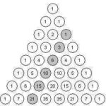
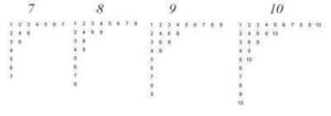
A surprisingly interesting structure is the extended multiplication table, shown above for the numbers seven to ten. The algorithm for drawing these is straight forward – for an n-extended table, start out as if you were writing a “regular” multiplication table, but extend each row so that it gets as close to, without exceeding, n. Another way to think about it is to write out rows of “skip counting up to n” by i for integers i from 1 to n.

This is called an extended multiplication table since it contains a “traditional” multiplication table inside it. The 12-extended table below contains a traditional 3×3 multiplication table.

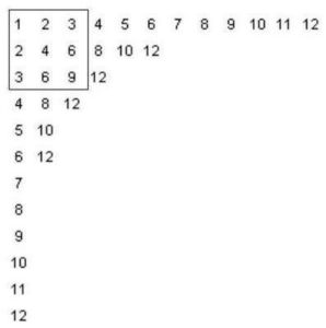
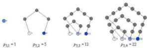
It turns out that 1 appears in an extended table once, and prime numbers appear exactly twice (once in the first column, and once in the first row). In general, for a natural number n, how many times does n appear in the n-extended table?

Before looking at that question, you might want to think about finding easier ways to draw the tables. Drawing out these tables by hand can be tedious – a simple program or spreadsheet might be easier. You can use Fathom, for example, to create the table data and draw it in the collections display. Create a slider m and the attributes listed in the table below (click on the image to see a larger version).

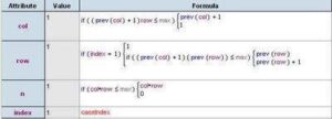
Modify the collection display attributes to draw the tables in the collection box. By adding lots of cases and using the slider m to filter out the ones you don’t need, you can vary the size of the table easily.

“how many times does n appear in the n-extended table?”

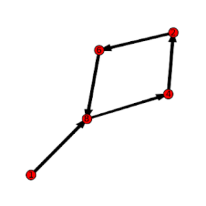
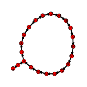
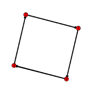
# of occurrances of n in the n-extended table = # of nodes in the factor lattice Fn

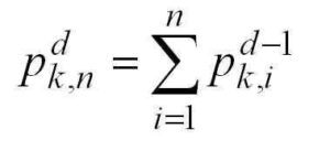
You can also recast both of these questions (how many occurances of n in the n-extended table, and how many nodesin the Fn factor lattice) as a combinatorial “balls in urns” problem.

Consider a set of colored balls where there are m different colours, where there are ki balls of color i, where i ranges from 1 to m. This would give a total number of balls equal to k1+k2+…+km. Suppose you were to distribute these balls in two urns. How many different distributions would there be? Using some counting techniques, you will find that the answer is (k1+1)*(k2+1)*…*(km+1).

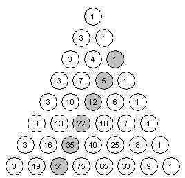
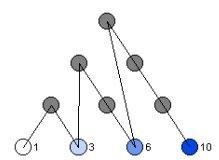
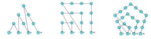
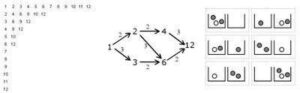
How is this connected to the other problems? Consider the prime factorization of the number. For each prime, choose a colour, and for each occurance of the prime in the factorization, add a new ball of that color. For example for 12 = 3*3*2, choose two colours – say blue=3 and red=2. Since 3 occurs twice and 2 occurs once, there should be two blue balls and one red ball. Now consider distributing these balls in two urns. It turns out that you get (2+1)*(1+1) = 6 possibilities. This is the same number of times 12 occurs in the 12-extended table, and the same number of nodes in the 12-factor lattice. The image below shows the 12-extended table, the 12-factor lattice, and the “ball and urn problem” for the numer 12.

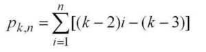
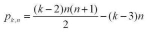
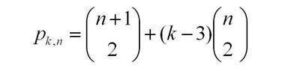
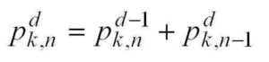
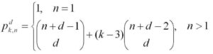
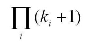
For a number n with the prime factorization:

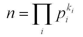
The answer to all three questions is given by:

For more such insights, log into www.international-maths-challenge.com.

*Credit for article given to dan.mackinnon*

Robert Recorde, author the first English textbook on algebra (published in 1557), chose to give his book the metaphorical title The Whetstone of Witte to encourage people to take up the new and difficult practice of algebra. The metaphor of a whetstone, or blade-sharpener, suggests that algebra is not only useful, but also good mental exercise. In the verse that he included on its title page, he writes,

Its use is great, and more than one. Here if you lift your wits to wet, Much sharpness thereby shall you get. Dull wits hereby do greatly mend, Sharp wits are fined to their full end.

Mathematics, and algebra in particular, according to The Whetstone of Witte is like a knife-sharpener for the brain. Four hundred years later, in his book Mathematician’s Delight (1961), W.W. Sawyer takes up a similar metaphor, suggesting that “Mathematics is like a chest of tools: before studying the tools in detail, a good workman should know the object of each, when it is used, how it is used.” Whether they describe mathematics as a sharpener or other tool, these mechanical metaphors are commonly used to emphasize the practicality and versatility of mathematics, particularly when employed in engineering or science, and suggest that it should be used thoughtfully, and with precision.

An often quoted mechanical metaphor that suggests a more frantic and less precise process of mathematical creation is often attributed to Paul Erdos: “a mathematician is a machine for turning coffee into theorems.”

For more such insights, log into www.international-maths-challenge.com.

*Credit for article given to dan.mackinnon*

 

Polygonal numbers are a mainstay of recreational and school mathematics, providing a nice bridge between numbers and shapes. The diagrams above show some of the hexagonal numbers.

Some examples of two-dimensional polygonal numbers are:

the triangular numbers: 1, 3, 6, 10, 15, …
the square numbers: 1, 4, 9, 16, 25, …
the pentagonal numbers: 1, 5, 12, 22, 35,…
the hexagonal numbers: 1, 6, 15, 28, 45, …

Comparing the listing for the hexagonal numbers with the diagrams above, you can see how the sequences are built diagrammatically. In general, beginning with a single dot, k-sided polygons are built by adding layers (called gnomons) consisting of k-2 segments, with each segment of the gnomon having one more dot than the segments of the previous layer. In this way, the nth gnomon consists of segments each n dots long, but with k-3 dots shared by adjoining segments (the corners).

The description above can lead you to a recursive formula for k-polygonals, writing p_k,n for the nth k-polygonal number:

Unwinding the recursion gives you a summation formula for k-polygonals:

Knowing a little about sums gives you the direct formula for k-polygonals:

Coming a little out of left-field is this combinatorial formula for k-polygonals:

This last formula expresses two ideas: that the triangular numbers correspond to the r=0 column of Pascal’s triangle, and that every polygonal number can be “triangulated”:

The combinatorial formula for p_kn can be generalized to higher-dimensional polygonal numbers (pyrimidal numbers, etc.).

The recreation here lies in showing that the various formulas for p_k,n are really the same, and then exploring the relationships between the different k-polygonals. A great resource is J.H. Conway and R.K. Guy’s The Book of Numbers.a

For more such insights, log into www.international-maths-challenge.com.

*Credit for article given to dan.mackinnon*

Looking at the last few digits that appear in the numbers that form the sequence b^0, b^1, b^2, b^3, … for b a positive integer, you’ll notice that the digits will always begin to repeat after a certain point. For example, looking at the last digit of the sequences for b = 2, 3, and 4 we have the sequences

b = 2: 1, 2, 4, 8, 6, 2, 4, 8, 6, …
b = 3: 1, 3, 9, 7, 1, 3, 9, 7, …
b = 4: 1, 4, 6, 4, 6, 4, 6, …

If we look at the sequence of last two digits of these sequence where b =2 we have

b = 2: 1, 2, 4, 8, 16, 32, 64, 28, 56, 12, 24, 48, 96, 92, 84, 68, 36, 72, 44, 88, 76, 52, 4, …

This sequence then repeats the loop that began at 4.

We can describe these sequences as T_b,d(n) = (b^n)mod 10^d. Recursively, T_b,d(n) = (T_b,d(n-1)*b)mod 10^d

These sequences are always eventually periodic. Although these sequences are simple to understand and calculate, there are several interesting ways of describing them.

For example, you can think of the elements of T_b,d as a commutative monoid, with multiplication defined as a*b = (a*b)mod 10^d. They form a monoid since 1 is always a member, and you can show that T_b,d is closed under the * operation. It turns out that for some values of b, and d, T_b,d is a group.

You can also think of this set as a finite state machine or graph, where each element is a node and the transition from one node to the next is defined by the operation *b mod 10^d. This provides a nice way of displaying the sequences. The pictures in this post were created by writing a short program to calculate the sequences, and then formatting the output to draw a di-graph in SAGE. The graph at the top of the post is for b=8, d=1, while the graph below is for b=2, d=2. The graph at the bottom of the page is for b=7, d=1.

For more such insights, log into www.international-maths-challenge.com.

*Credit for article given to dan.mackinnon*

The third diagonal column in Pascal’s Triangle (r = 2 in the usual way of labeling and numbering) consists of the triangular numbers (1, 3, 6, 10, …) – numbers that can be arranged in 2-dimensional triangular patterns. The fourth column of Pascal’s triangle gives us triangular-based pyramidal numbers (1, 4, 10, 20, …), built by stacking the triangular numbers. The columns further out give “higher dimensional” triangular numbers that arise from stacking the triangular numbers from the previous dimension.

It is not by coincidence that the triangular and higher-dimensional triangular numbers appear in Pascal’s Triangle. If you think about layering of polygonal numbers in terms of equations, you get

In the above equation p^d_(k,n) is the nth k-polygonal number of dimension d. Triangular numbers are the 3-polygonal numbers of dimension 2, square numbers are the 4-polygonal numbers of dimension 2, “square based pyramidal numbers” would be denoted as p^3_(4,n).
from the sum above, you can obtain this equation:

Which looks very much like the Pascal Identity C(n,r) = C(n-1,r-1) + C(n-1,r), except for some translation of the variables. To be precise, if we consider the case where k=3 and use r = d and n‘ = n+d-1 we can translate the triangular numbers into the appropriate positions in Pascal’s Triangle.

Along with the definitions for the end columns, the Pascal Identity allows us to generate the whole triangle. This suggests the following strategy for calculating the higher k-Polygonal numbers: create a modified Pascal’s Triangle whose first column is equal to k-2 (instead of 1), and whose last column is equal to 1 (as usual). This modified Pascal’s Triangle is generated using these initial values and the usual Pascal Identity.

Here is an example with k=5, which sets the first column values equal to 3 (except for the top value, which we keep as 1) and yields the pentagonal numbers (column 3) and the higher pentagonal numbers.

The formula for these modified Pascal Triangles is given by this equation:

If we apply the change of variables mentioned above, we can obtain this general formula for the higher polygonal numbers in terms of combinations:

This formula illustrates how polygonal numbers are built out of triangular numbers. It says that the nth d-dimensional k-polygonal number is equal to the nth d-dimensional triangular number, plus (k-3) copies of the n-1 d-dimensional triangular number. This is a little easier to understand when you forget about the higher-dimensions and look at the regular 2-dimensional polygonal number.

For more such insights, log into www.international-maths-challenge.com.

*Credit for article given to dan.mackinnon*

 

John Sims has created a number of pi-related art works. One, the Pi Color Map, can be recreated effectively using TinkerPlots. The image above is one such Pi Color Map, using 2281 digits of pi.

Here are some instructions for creating a Pi Color Map in Tinkerplots.

1. Obtain a listing of the digits of pi – up to a reasonable number. You can get the digits from several sites, including the pi day site.

2. Paste your listing to a text document, and get them arranged into a single column. One strategy for doing this is and use the find/replace feature of a word-processor to replace each number with the number itself plus a line-break(e.g. in Word, replace 2 with 2^l, etc.).

3. If you’ve included the decimal point, remove it. For the first line of your document, provide a heading like pi_expansion. This will be your TinkerPlots attribute.

3. Import the text file into TinkerPlots using the File>Import menu.

4. Create a new attribute called digit whose formula is digit=concat(“”,pi_expansion). This creates a categorical data type that TinkerPlots won’t treat numerically. This is what you will use as your color key. Using the pi_expansion attribute gives a spectrum of color, rather than distinct colors for each number.

5. Create a new attribute called place, whose formula is place=caseIndex. This is what you will order your plot by.

6. Create a new plot, lock the color key on the digit attribute. Select the place attribute and press the Order By button.

7. Change your icon type to small squares, and stack the cases.

You can play with different options to get different effects for your color map.

One nice thing about doing this in TinkerPlots is that you can investigate the data further. The color map plot highlights the apparent randomness of the pi expansion, but you can also create other attributes and plots to investigate things like the running average of the digits, occurrences of consecutive digits, and the overall distribution of the digits (it should be uniform).

For more such insights, log into www.international-maths-challenge.com.

*Credit for article given to dan.mackinnon*

 

If You take a look at the square numbers (n^2, n a positive integer), you’ll notice plenty of patterns in the digits. For example, if you look at just the last digit of each square, you’ll observe the repeating pattern 1, 4, 9, 6, 5, 6, 9, 4, 1, 0, … If you construct a graph of “last digit” vs n (like the one below, built with Falthom), the symmetry and period of this digit pattern is apparent.

Why does this happen? The periodic nature of the pattern is easy to understand – when you square a number, only the digit in the ones place contributes to ones place of the product. For example, 22*22 and 32*32 are both going to have a 4 as their last digit – the values in the tens place (or any other place other than the ones) do not affect what ends up as the last digit.

The reason for the symmetry about n=5 is a little less obvious. To see what is going on, it is helpful to use modular arithmetic and to realize that ” last digit of n” is the same as “n mod 10”. Considering what 10-n looks like mod 10 after it is squared, we have the equation below.

This tells us that the last digit of (10-n)^2 is the same as the last digit of n^2, because everything else that is different about these two numbers is divisible by 10.

If you look at the last two digits of the square numbers, you see another repeating pattern that has similar symmetries.

This is a nice looking graph – the period is 50 with a line of symmetry at n=25. You can think about it in the same way as the one-digit case, this time the symmetry is understood by looking at (50-n)^2 mod 100. (Looking at numbers mod 100 tells us their last two digits.)

If you decide to investigate patterns in cubes or higher powers, you’ll see somewhat similar results. Using the binomial theorem and modular arithmetic, you can see why even powers give symmetry similar to the n^2 case, while odd powers do not (although all are periodic).

This graph shows the pattern in the last digit of n^3.

This last graph shows the pattern for the last two digits of n^4.

For more such insights, log into www.international-maths-challenge.com.

*Credit for article given to dan.mackinnon*

The diagram above (known as the tetractys) shows the first four triangular numbers (1, 3, 6, 10, …). Although there is a simple formula for calculating these numbers directly, t(n) = 1/2(n(n+1)), constructing them by these layered-triangle diagrams helps to show their geometric and recursive properties.

More generally, polygonal numbers arise from counting arrangements of dots in regular polygonal patterns. Larger polygons are built from smaller ones of the same type by adding additional layers of dots, called gnomons. Beginning with a single dot, k-sided polygons are built by adding gnomons consisting of k-2 segments, with each segment of the gnomon having one more dot than the segments of the previous layer. In this way, the nth gnomon consists of segments each n dots long, but with k-3 dots shared by adjoining segments (the corners).

This post describes how you can draw figures that illustrate the polygonal numbers and explore the polygonal numbers in general (triangular, square, pentagonal, hexagonal, etc.) using either TinkerPlots or Fathom. Both TinkerPlots and Fathom work well, but TinkerPlots creates nicer pictures, and allows for captions directly on the graph.
Without describing the details of how you create Fathom or TinkerPlot documents, here are the attributes that you will want to define in order to draw diagrams like the ones shown.

Required attributes
Create a slider k. This will allow you to set what kind of polygonal number you want to draw (k=3 gives triangular numbers, k=4 gives square numbers, etc.)
Define the following attributes:

n The number itself. This is a natural number beginning at 1 and continuing through the number of cases.

gnomon This states which “layer” or gnomon the number belongs in. It is calculated based on a number of other attributes.

g_index This is the position of the number within the gnonom – it ranges from 1 up until the next k-polygonal number is hit.

s_index Each gonom is broken up into sections or sides – what is the position within the side? Each side is of length equal to the gonom number. The first gonom has sides of length 1, the second has length 2, etc.

corner This keeps track of whether or not the number is a “corner” or not. This is based primarily on the s_index attribute.

c_index This keeps track of how many corners we have so far. There are only k-1 corners in a gnomon (the first number n=1 is the remaining corner). So, when we hit the last corner, we know we are at a polygonal number.

k_poly Records whether or not the number n is k-polygonal. It does this by checking to see if it is the last corner of a gnonom.
The attributes listed above are required for finding the position of each number within the figure; th following attributes are used in actually drawing the figures.

angle The base corner angle for the polygon is determined by k. This is the external angle for each corner.

current_angle We have to add to the base angle at each corner as we turn at each corner. This attribute is used to keep track of the total current angle.

dx This is the x-component of the unit direction vector that we are travelling in. Each new dot moves one dx over in the x-direction. It is given by the cosine of the current angle.

dy This is the y-component of the unit direction vector that we are travelling in. Each new dot moves one dy over in the y-direction. It is given by the sine of the current angle.

prev_g_1_x This is the x-coordinate of the first dot in the previous gonom layer. We need to know this because it will be the starting point for the next layer – each layer starts back at the “beginning” of the figure.

prev_g_1_y This is the y- coordinate of the first dot in the previous gonom layer.

x This is the x-coordinate of the current dot, calculated either from the previous dot or from the first dot in the previous layer.

y This is the y-coordinate of the current dot, calculated either from the previous dot or from the first dot in the previous layer.

caption Used to display the number on the plot (TinkerPlots only)
Below are the formulas for each attribute, written in “ascii” math. They are presented without a full explanation, in the hopes that if you try to implement this you will think about and explore each using the formulas and the descriptions above as a guide. Alternate methods for drawing the diagrams are possible, and you might find other formulas that achieve the same goals. Note that there are nested if() statements in several formulas.

n = caseIndex

gnomon = if(n=1){1, if(prev(k_poly)){prev(gnomon)+1, prev(gnomon)

g_index = if(n=1){ 1, if(prev(k_poly){1, prev(g_index) +1

s_index = if(n=1){ 1, if(prev(k_poly){1, if(prev(s_index) = gnomon){2,prev(s_index)

corner = (s_index=1) or (s_index=gnomon)

c_index= if(g_index=1){1, if(corner){prev(c_index)+1, prev(c_index)

k_poly = if(n=1){true, (c_index=k-1)

prev_g_1_x = if (n=1){0, if(g_index=2){prev(x), prev(prev_g_1_x)

prev_g_1_y = if(n=1){0, if(g_index=2){prev(y), prev(prev_g_1_y)

angle = pi-((k-2)*(pi/k))

current_angle = if(g_index =1) {pi-angle, if(pref(corner)){prev(current_angle)-angle, prev(current_angle)

dx = cos(current_angle)

dy = sin(current_angle)

x= if(n=1){0, if(g_index=1){prev_g_1_x +dx, prev(x) +dx

y =if(n=1){0, if(g_index=1){prev_g_1_y +dy, prev(y) +dy

caption = if(k_poly){n,””

To actually draw the diagrams, create a new plot with the x and y attributes as the horizontal and vertical axis, respectively. Add cases to the collection to populate the diagram. Optionally you can show connecting lines, and (in TinkerPlots) add a legend using the caption attribute.

For more such insights, log into www.international-maths-challenge.com.

*Credit for article given to dan.mackinnon*

See a vertical stripe, what you are seeing is a run of repeated digits, like 7777, 00000, or 222.

One occurs in the top left:

Sequences like this used to be important examples in motivating discussions about the law of the excluded middle. Statements like: ‘the decimal expansion of pi contains the sequence 7777’, according to the law of the excluded middle, are either true or false. But when you are discussing something that has never been calculated, and that might never be calculated, suggests (to constructivists), that the statement may be neither true or false, and that the sequence 7777 may be somewhat like Schrodinger’s cat, neither existing nor not existing.

Now that the digits of pi have been calculated to astounding lengths, and that mathematics exists to uncover the properties of the pi digit sequence, the expansion of pi is no longer an ideal candidate for constructivist thought experiments. Even some exotic questions about the decimal expansion of pi, like the convergence of the brouwer-heyting sequence, have been resolved. Questions about the expansion of pi that illustrate constructivist problems can still be formulated, but they need to be more complicated than they used to be.

Still, I decided to look more closely at this little sequence that occurs (relatively) early on in the pi expansion. The stripe in the pi colour map mentioned above corresponds to the sequence 999999 beginning at digit 763 and ending at digit 768. This was observed in a set of the first 2281 digits of pi.

I decided to push the software a bit further, and load 10000 digits of pi into the document.  (A file with the first 10000 digits of pi formatted for Fathom or TinkerPlots is here.) The plot below shows the digits with 9 in black and all other digits blanked out – dots are single occurrences of a 9, while vertical stripes are runs of repeated 9s.

Using Tinkerplots’ runLength function we can see how frequent runs of various lengths are, and easily identify the longer ones.

Even with 10000 digits, the 999999 sequence at digit 763 was still the longest sequence of repeated digits. The other runner-up sequences in this first 10000 digits are, two instances of 2222, a single run of 8888, and four distinct occurrences of 7777.

The plot at the bottom of this post shows the distribution of even and odd digits in the decimal expansion of pi’s first 10000 digits, and was inspired by a similar plot from Wolfram Math World.

For more such insights, log into www.international-maths-challenge.com.

*Credit for article given to dan.mackinnon*