Month: March 2018

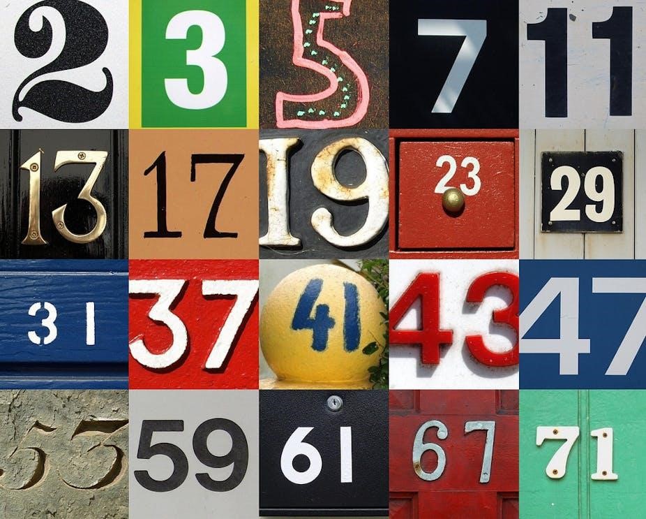
What will be the next number in this sequence?

“At school I was never really good at maths” is an all too common reaction when mathematicians name their profession.

In view of most people’s perceived lack of mathematical talent, it may come as somewhat of a surprise that a recent study carried out at John Hopkins University has shown that six-month-old babies already have a clear sense of numbers. They can count, or at least approximate, the number of happy faces shown on a computer screen.

By the time they start school, at around the age of five, most children are true masters of counting, and many will proudly announce when for the first time they have counted up to 100 or 1000. Children also intuitively understand the regular nature of counting; by adding sufficiently many ones to a starting value of one they know they will eventually reach their own age, that of their parents, grandparents, 2011, and so on.

Counting is child’s play. Photography By Shaeree

From counting to more general addition of whole numbers is only a small step—again within children’s almost-immediate grasp. After all, counting is the art of adding one, and once that is mastered it takes relatively little effort to work out that 3 + 4 = 7. Indeed, the first few times children attempt addition they usually receive help from their fingers or toes, effectively reducing the problem to that of counting:

3 + 4 = (1 + 1 + 1) + (1 + 1 + 1 + 1) = 7.

For most children, the sense of joy and achievement quickly ends when multiplication enters the picture. In theory it too can be understood through counting: 3 x 6 is three lots of six apples, which can be counted on fingers and toes to give 18 apples.

In practice, however, we master it through long hours spent rote-learning multiplication tables—perhaps not among our favourite primary school memories.

But at this point, we ask the reader to consider the possibility—in fact, the certainty—that multiplication is far from boring and uninspiring, but that it is intrinsically linked with some of mathematics’ deepest, most enduring and beautiful mysteries. And while a great many people may claim to be “not very good at maths” they are, in fact, equipped to understand some very difficult mathematical questions.

Primes

Let’s move towards these questions by going back to addition and those dreaded multiplication tables. Just like the earlier example of 7, we know that every whole number can be constructed by adding together sufficiently many ones. Multiplication, on the other hand, is not so well-behaved.

The number 12, for example, can be broken up into smaller pieces, or factors, while the number 11 cannot. More precisely, 12 can be written as the product of two whole numbers in multiple ways: 1 x 12, 2 x 6 and 3 x 4, but 11 can only ever be written as the product 1 x 11. Numbers such as 12 are called composite, while those that refuse to be factored are known as prime numbers or simply primes. For reasons that will soon become clear, 1 is not considered a prime, so that the first five prime numbers are 2, 3, 5, 7 and 11.

Just as the number 1 is the atomic unit of whole-number addition, prime numbers are the atoms of multiplication. According to the Fundamental Theorem of Arithmetic, any whole number greater than 1 can be written as a product of primes in exactly one way. For example: 4 = 2 x 2, 12 = 2 x 2 x 3, 2011 = 2011 and

13079109366950 = 2 x 5 x 5 x 11 x 11 x 11 x 37 x 223 x 23819,

where we always write the factors from smallest to largest. If, rather foolishly, we were to add 1 to the list of prime numbers, this would cause the downfall of the Fundamental Theorem of Arithmetic:

4 = 2 x 2 = 1 x 2 x 2 = 1 x 1 x 2 x 2 = …

In the above examples we have already seen several prime numbers, and a natural question is to ask for the total number of primes. From what we have learnt about addition with its single atom of 1, it is not unreasonable to expect there are only finitely many prime numbers, so that, just maybe, the 2649th prime number, 23819, could be the largest. Euclid of Alexandria, who lived around 300BC and who also gave us Euclidean Geometry, in fact showed that there are infinitely many primes.

Euclid’s reasoning can be captured in just a single sentence: if the list of primes were finite, then by multiplying them together and adding 1 we would get a new number which is not divisible by any prime on our list—a contradiction.

A few years after Euclid, his compatriot Eratosthenes of Cyrene found a clever way, now known as the Sieve of Eratosthenes, to obtain all primes less than a given number.

For instance, to find all primes less than 100, Eratosthenes would write down a list of all numbers from 2 to 99, cross out all multiples of 2 (but not 2 itself), then all multiples of 3 (but not 3 itself), then all multiples of 5, and so on. After only four steps(!) this would reveal to him the 25 primes

2, 3, 5, 7, 11, 13, 17, 19, 23, 29, 31, 37, 41, 43, 47, 53, 59, 61, 67, 71, 73, 79, 83, 89 and 97.

While this might seem very quick, much more sophisticated methods, combined with very powerful computers, are needed to find really large prime numbers. The current world record, established 2008, is the truly monstrous 2^43112609 – 1, a prime number of approximately 13 million digits.

The quest to tame the primes did not end with the ancient Greeks, and many great mathematicians, such as Pierre de Fermat, Leonhard Euler and Carl Friedrich Gauss studied prime numbers extensively. Despite their best efforts, and those of many mathematicians up to the present day, there are many more questions than answers concerning the primes.

One famous example of an unsolved problem is Goldbach’s Conjecture. In 1742, Christian Goldbach remarked in a letter to Euler that it appeared that every even number greater than 2 could be written as the sum of two primes.

For example, 2012 = 991 + 1021. While computers have confirmed the conjecture holds well beyond the first quintillion (10¹⁸) numbers, there is little hope of a proof of Goldbach’s Conjecture in the foreseeable future.

Another intractable problem is that of breaking very large numbers into their prime factors. If a number is known to be the product of two primes, each about 200 digits long, current supercomputers would take more than the lifetime of the universe to actually find these two prime factors. This time round our inability to do better is in fact a blessing: most secure encryption methods rely heavily on our failure to carry out prime factorisation quickly. The moment someone discovers a fast algorithm to factor large numbers, the world’s financial system will collapse, making the GFC look like child’s play.

To the dismay of many security agencies, mathematicians have also failed to show that fast algorithms are impossible—the possibility of an imminent collapse of world order cannot be entirely ruled out!

Margins of error

For mathematicians, the main prime number challenge is to understand their distribution. Quoting Don Zagier, nobody can predict where the next prime will sprout; they grow like weeds among the whole numbers, seemingly obeying no other law than that of chance. At the same time the prime numbers exhibit stunning regularity: there are laws governing their behaviour, obeyed with almost military precision.

The Prime Number Theorem describes the average distribution of the primes; it was first conjectured by both Gauss and Adrien-Marie Legendre, and then rigorously established independently by Jacques Hadamard and Charles Jean de la Vallée Poussin, a hundred years later in 1896.

The Prime Number Theorem states that the number of primes less than an arbitrarily chosen number n is approximately n divided by ln(n), where ln(n) is the natural logarithm of n. The relative error in this approximation becomes arbitrarily small as n becomes larger and larger.

For example, there are 25 primes less than 100, and 100/ln(100) = 21.7…, which is around 13% short. When n is a million we are up to 78498 primes and since 10⁶/ln(10⁶) = 72382.4…, we are only only 8% short.

The Riemann Hypothesis

The Prime Number Theorem does an incredible job describing the distribution of primes, but mathematicians would love to have a better understanding of the relative errors. This leads us to arguably the most famous open problem in mathematics: the Riemann Hypothesis.

Posed by Bernhard Riemann in 1859 in his paper “Ueber die Anzahl der Primzahlen unter einer gegebenen Grösse” (On the number of primes less than a given magnitude), the Riemann Hypothesis tells us how to tighten the Prime Number Theorem, giving us a control of the errors, like the 13% or 8% computed above.

The Riemann Hypothesis does not just “do better” than the Prime Number Theorem—it is generally believed to be “as good as it gets”. That is, we, or far-superior extraterrestrial civilisations, will never be able to predict the distribution of the primes any better than the Riemann Hypothesis does. One can compare it to, say, the ultimate 100 metres world record—a record that, once set, is impossible to ever break.

Finding a proof of the Riemann Hypothesis, and thus becoming record holder for all eternity, is the holy grail of pure mathematics. While the motivation for the Riemann Hypothesis is to understand the behaviour of the primes, the atoms of multiplication, its actual formulation requires higher-level mathematics and is beyond the scope of this article.

In 1900, David Hilbert, the most influential mathematician of his time, posed a now famous list of 23 problems that he hoped would shape the future of mathematics in the 20th century. Very few of Hilbert’s problems other than the Riemann Hypothesis remain open.

Inspired by Hilbert, in 2000 the Clay Mathematics Institute announced a list of seven of the most important open problems in mathematics. For the successful solver of any one of these there awaits not only lasting fame, but also one million US dollars in prize money. Needless to say, the Riemann Hypothesis is one of the “Millennium Prize Problems”.

Hilbert himself remarked: “If I were awoken after having slept for a thousand years, my first question would be: has the Riemann Hypothesis been proven?” Judging by the current rate of progress, Hilbert may well have to sleep a little while longer.

For more such insights, log into www.international-maths-challenge.com.

*Credit for article given to Ole Warnaar*

 

Let’s talk numbers for a moment.

The moon is approximately 384,000 kilometres away, and the sun is approximately 150 million kilometres away. The mean distance between Earth and the sun is known as the “astronomical unit” (AU). Neptune, the most distant planet, then, is 30 AU from the sun.

The nearest stars to Earth are 1,000 times more distant, roughly 4.3 light-years away (one light-year being the distance that light travels in 365.25 days – just under 10 trillion kilometres).

The Milky Way galaxy consists of some 300 billion stars in a spiral-shaped disk roughly 100,000 light-years across.

The Andromeda Galaxy, which can be seen with many home telescopes, is 2.54 million light years away. There are hundreds of billions of galaxies in the observable universe.

At present, the most distant observed galaxy is some 13.2 billion light-years away, formed not long after the Big Bang, 13.75 billion years ago (plus or minus 0.011 billion years).

The scope of the universe was illustrated by the astrophysicist Geraint Lewis in a recent Conversation article.

He noted that, if the entire Milky Way galaxy was represented by a small coin one centimetre across, the Andromeda Galaxy would be another small coin 25 centimetres away.

Going by this scale, the observable universe would extend for 5 kilometres in every direction, encompassing some 300 billion galaxies.

But how can scientists possibly calculate these enormous distances with any confidence?

Parallax

One technique is known as parallax. If you cover one eye and note the position of a nearby object, compared with more distant objects, the nearby object “moves” when you view it with the other eye. This is parallax (see below).

The same principle is used in astronomy. As Earth travels around the sun, relatively close stars are observed to move slightly, with respect to other fixed stars that are more distant.

Distance measurements can be made in this way for stars up to about 1,000 light-years away.

Standard candles

For more distant objects such as galaxies, astronomers rely on “standard candles” – bright objects that are known to have a fixed absolute luminosity (brightness).

Since light flux falls off as the square of the distance, by measuring the actual brightness observed on Earth astronomers can calculate the distance.

One type of standard candle, which has been used since the 1920s, is Cepheid variable stars.

Distances determined using this scheme are believed accurate to within about 7% for more nearby galaxies, and 15-20% for the most distant galaxies.

Type Ia supernovas

In recent years scientists have used Type Ia supernovae. These occur in a binary star system when a white dwarf star starts to attract matter from a larger red dwarf star.

As the white dwarf gains more and more matter, it eventually undergoes a runaway nuclear explosion that may briefly outshine an entire galaxy.

Because this process can occur only within a very narrow range of total mass, the absolute luminosity of Type Ia supernovas is very predictable. The uncertainty in these measurements is typically 5%.

In August, worldwide attention was focused on a Type Ia supernova that exploded in the Pinwheel Galaxy (known as M101), a beautiful spiral galaxy located just above the handle of the Big Dipper in the Northern Hemisphere. This is the closest supernova to the earth since the 1987 supernova, which was visible in the Southern Hemisphere.

These and other techniques for astronomical measurements, collectively known as the “cosmic distance ladder”, are described in an excellent Wikipedia article. Such multiple schemes lend an additional measure of reliability to these measurements.

In short, distances to astronomical objects have been measured with a high degree of reliability, using calculations that mostly employ only high-school mathematics.

Thus the overall conclusion of a universe consisting of billions of galaxies, most of them many millions or even billions of light-years away, is now considered beyond reasonable doubt.

Right tools for the job

The kind of distances we’re dealing with above do cause consternation for some since, as we peer millions of light-years into space, we are also peering millions of years into the past.

Some creationists, for instance, have theorised that, in about 4,000 BCE, a Creator placed quadrillions of photons in space en route to Earth, with patterns suggestive of supernova explosions and other events millions of years ago.

Needless to say, most observers reject this notion. Kenneth Miller of Brown University commented, “Their [Creationists’] version of God is one who has filled the universe with so much bogus evidence that the tools of science can give us nothing more than a phony version of reality.”

There are plenty of things in the universe to marvel at, and plenty of tools to help us understand them. That should be enough to keep us engaged for now.

For more such insights, log into our website https://international-maths-challenge.com

Credit of the article given to Jonathan Borwein (Jon), University of Newcastle and David H. Bailey, University of California, Davis

This knot has Gauss code O1U2O3U1O2U3. Credit: Graphic by Sam Nelson.

In the 19th century, Lord Kelvin made the inspired guess that elements are knots in the “ether”. Hydrogen would be one kind of knot, oxygen a different kind of knot—and so forth throughout the periodic table of elements. This idea led Peter Guthrie Tait to prepare meticulous and quite beautiful tables of knots, in an effort to elucidate when two knots are truly different. From the point of view of physics, Kelvin and Tait were on the wrong track: the atomic viewpoint soon made the theory of ether obsolete. But from the mathematical viewpoint, a gold mine had been discovered: The branch of mathematics now known as “knot theory” has been burgeoning ever since.

In his article “The Combinatorial Revolution in Knot Theory”, to appear in the December 2011 issue of the Notices of the AMS, Sam Nelson describes a novel approach to knot theory that has gained currency in the past several years and the mysterious new knot-like objects discovered in the process.

As sailors have long known, many different kinds of knots are possible; in fact, the variety is infinite. A *mathematical* knot can be imagined as a knotted circle: Think of a pretzel, which is a knotted circle of dough, or a rubber band, which is the “un-knot” because it is not knotted. Mathematicians study the patterns, symmetries, and asymmetries in knots and develop methods for distinguishing when two knots are truly different.

Mathematically, one thinks of the string out of which a knot is formed as being a one-dimensional object, and the knot itself lives in three-dimensional space. Drawings of knots, like the ones done by Tait, are projections of the knot onto a two-dimensional plane. In such drawings, it is customary to draw over-and-under crossings of the string as broken and unbroken lines. If three or more strands of the knot are on top of each other at single point, we can move the strands slightly without changing the knot so that every point on the plane sits below at most two strands of the knot. A planar knot diagram is a picture of a knot, drawn in a two-dimensional plane, in which every point of the diagram represents at most two points in the knot. Planar knot diagrams have long been used in mathematics as a way to represent and study knots.

As Nelson reports in his article, mathematicians have devised various ways to represent the information contained in knot diagrams. One example is the Gauss code, which is a sequence of letters and numbers wherein each crossing in the knot is assigned a number and the letter O or U, depending on whether the crossing goes over or under. The Gauss code for a simple knot might look like this: O1U2O3U1O2U3.

In the mid-1990s, mathematicians discovered something strange. There are Gauss codes for which it is impossible to draw planar knot diagrams but which nevertheless behave like knots in certain ways. In particular, those codes, which Nelson calls *nonplanar Gauss codes*, work perfectly well in certain formulas that are used to investigate properties of knots. Nelson writes: “A planar Gauss code always describes a [knot] in three-space; what kind of thing could a nonplanar Gauss code be describing?” As it turns out, there are “virtual knots” that have legitimate Gauss codes but do not correspond to knots in three-dimensional space. These virtual knots can be investigated by applying combinatorial techniques to knot diagrams.

Just as new horizons opened when people dared to consider what would happen if -1 had a square root—and thereby discovered complex numbers, which have since been thoroughly explored by mathematicians and have become ubiquitous in physics and engineering—mathematicians are finding that the equations they used to investigate regular knots give rise to a whole universe of “generalized knots” that have their own peculiar qualities. Although they seem esoteric at first, these generalized knots turn out to have interpretations as familiar objects in mathematics. “Moreover,” Nelson writes, “classical knot theory emerges as a special case of the new generalized knot theory.”

For more such insights, log into our website https://international-maths-challenge.com

Credit of the article given to American Mathematical Society

 

My intention with this article is to give an intuitive and non-technical introduction to the field of evolutionary algorithms, particularly with regards to optimisation.

If I get you interested, I think you’re ready to go down the rabbit hole and simulate evolution on your own computer. If not … well, I’m sure we can still be friends.

Survival of the fittest

According to Charles Darwin, the great evolutionary biologist, the human race owes its existence to the phenomenon of survival of the fittest. And being the fittest doesn’t necessarily mean the biggest physical presence.

Once in high school, my lunchbox was targeted by swooping eagles, and I was reduced to a hapless onlooker. The eagle, though smaller in form, was fitter than me because it could take my lunch and fly away – it knew I couldn’t chase it.

As harsh as it sounds, look around you and you will see many examples of the rule of the jungle – the fitter survive while the rest gradually vanish.

The research area, now broadly referred to as Evolutionary Algorithms, simulates this behaviour on a computer to find the fittest solutions to a number of different classes of problems in science, engineering and economics.

The area in which this area is perhaps most widely used is known as “optimisation”.

Optimisation is everywhere

Your high school maths teacher probably told you the shortest way to go from point A to point B was along the straight line joining A and B. Your mum told you that you should always get the right amount of sleep.

And, if you have lived on your own for any length of time, you’ll be familiar with the ever-increasing cost of living versus the constant income – you always strive to minimise the expenditures, while ensuring you are not malnourished.

Whenever you undertake an activity that seeks to minimise or maximise a well-defined quantity such as distance or the vague notion of the right amount of sleep, you are optimising.

Look around you right now and you’ll see optimisation in play – your Coke can is shaped like that for a reason, a water droplet is spherical for a reason, you wash all your dishes together in the dishwasher for a reason.

Each of these strives to save on something: volume of material of the Coke can, and energy and water, respectively, in the above cases.

So we can safely say optimisation is the act of minimising or maximising a quantity. But that definition misses an important detail: there is always a notion of subject to, or satisfying some conditions.

You must get the right amount of sleep, but you also must do your studies and go for your music lessons. Such conditions, which you also have to adhere to, are known as “constraints”. Optimisation with constraints is then collectively termed “constrained optimisation”.

After constraints comes the notion of “multi-objective optimisation”. You’ll usually have more than one thing to worry about (you must keep your supervisor happy with your work and keep yourself happy and also ensure that you are working on your other projects). In many cases these multiple objectives can be in conflict.

Evolutionary algorithms and optimisation

Imagine your local walking group has arranged a weekend trip for its members and one of the activities is a hill climbing exercise. The problem assigned to your group leader is to identify who among you will reach the hill in the shortest time.

There are two approaches he or she could take to complete this task: ask only one of you to climb up the hill at a time and measure the time needed, or ask all of you to run all at once and see who reaches first.

That second method is known as the “population approach” of solving optimisation problems – and that’s how evolutionary algorithms work. The “population” of solutions are evolved over a number of iterations, with only the fittest solutions making it to the next.

This is analogous to the champion girl from your school making to the next round which was contested among champions from other schools in your state, then your country, and finally winning among all the countries.

Or, in our above scenario, finding who in the walking group reaches the hill top fastest, who would then be denoted as the fittest.

In engineering, optimisation needs are faced at almost every step, so it’s not surprising evolutionary algorithms have been successful in that domain.

Design optimisation of scramjets

At the Multi-disciplinary Design Optimisation Group at the University of New South Wales, my colleagues and I are involved in the design optimisation of scramjets, as part of the SCRAMSPACE program. In this, we’re working with colleagues from the University of Queensland.

Our evolutionary algorithms-based optimisation procedures have been successfully used to obtain the optimal configuration of various components of a scramjet.

Some of these have quite technical names, that in themselves would require quite a bit of explanation but, if you want, you can get a feel for the kind of work we do, and its applications for scramjets, by clicking here.

There are, at the risk of sounding over-zealous, no limits to the application of evolutionary algorithms.

Has this whetted your appetite? Have you learnt something new today?

If so, I’m glad. May the force be with you!

For more such insights, log into www.international-maths-challenge.com.

*Credit for article given to Amit Saha*