Month: August 2017

With connections to the study of gambling, Brownian motion, fractals, and more, random walks are a favourite topic in recreational mathematics.

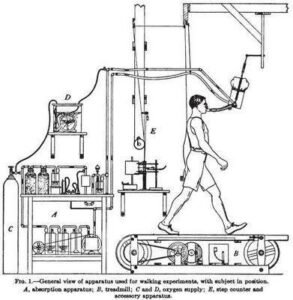
The diagram above (from Energy transformations during horizontal walking by F. G. Benedict and H. Murschhauser, published in 1915) suggests one method for generating walking data. Creating random walk simulations in Fathom or TinkerPlots is a little more straightforward.

First simulation – using sliders to determine a ‘base angle’

This first example lets you set up random walks where the direction chosen is based on an angle k*2pi/n for a fixed n (whose value is determined by a slider) and a random k (a random integer between 1 and n).

First, create a slider n, then create the attributes below and finally add the data (any number is fine – start with ~500 cases). The formulas below were entered in TinkerPlots, but would work equally well in Fathom.

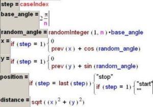
Plots of (x,y) will show the walk, and plots of (step, distance) will show how the distance from the origin changes over the course of the walk. Different values for n provide walks with their own particular geometries.

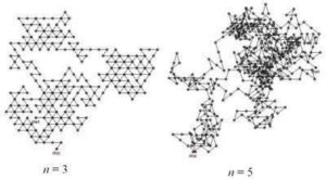
The walks start at (0,0) and wander about the plane from there. Re-randomizing (CNTRL-Y) generates new walks.

The simulation gives lots of nice pictures of random walks. You could generate statistics from these by adding measures and measure collections.

One limitation of this simulation is that it is difficult to determine exactly when the walker has returned to the start (0,0).  This turns out to be an interesting question for random walks on the plane (see the wikipedia entry for more on this). Because of the inexactness in the positions calculated using sine and cosine, the walker seems to never return to the origin. There are several ways of dealing with this, but one is to design a simpler simulation that uses exact values – one that sticks to lattice points (x, y), where x and y are both integers.

Second simulation – sticking to Integer lattice points

This second simulation can be thought of an ‘urban walker’ where all paths must follow a strictly laid out grid, like some downtown streets. The exactness of the positions means that we can detect with confidence when the walker has crossed back to their starting point. For this simulation, no slider is required – just enter the attributes and add cases.

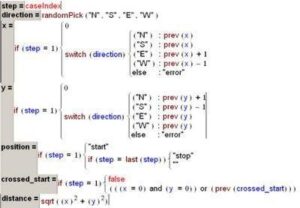
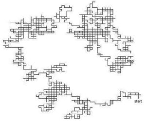
Using the crossed_start attribute as a filter or to gather measures, you will find that walks often quickly pass over the starting point. You will also find that as you increase the number of cases, the straight ‘etch-a-sketch’ lines of the urban walk take on very interesting fractal-like contours.

For more such insights, log into www.international-maths-challenge.com.

*Credit for article given to dan.mackinnon*

It could be argued that the square is the ‘nicest’ rhombus, but the rhombus with angles of 60 and 120 degrees seems nicer still. One of the nice things about the 60/120 rhomb are the plane tilings that can be constructed from it. One of these tilings is the ‘tumbling blocks’ tiling shown at the top of the post, in which at some points you see ‘cubes’ (around the degree 3 vertices), while at others you see ‘flowers’ (around the degree 6 vertices). Because of the two different types of vertices, this is known as a quasi-regular rhombic tiling. (Another tiling that uses the 60/120 rhomb is this one.)

If you want to build a polyhedron that resembles the tumbling block tiling, one method is to reduce the number of petals in your flowers to 5, and then stretch your 60/120 rhombs until they are have angles of 63.435 and 116.565 degrees. Thirty of these rhombs arranged around vertices of degree 3 and 5 produces a quasi-regular polygon known as the rhombic triacontahedron.

The image above is of a model that was built using rhombic units printed onto card stock.

Despite the apparent ugliness of the 63.435 and 116.565 degree angle-measurements, our nice 60/120 rhomb has been, arguably, stretched into an even nicer one – a ‘golden rhombus,’ so called because the ratio of the diagonals is equal to the golden ratio.

The dual of the rhombic triacontahedron is the archemedian polyhedron known as the icosidodecahedron.

For more such insights, log into www.international-maths-challenge.com.

*Credit for article given to dan.mackinnon*

The diagram above illustrates a surprising correspondence – if you take the reciprocal of a particular polynomial whose coefficients match the d+1 row of Pascal’s Triangle, you obtain a formal power series whose coefficients are precisely the elements in the dth column of the triangle.

The case for the third row is shown above (row and column numbering starts at 0 in Pascal’s Triangle), and the case for the fourth row is shown in the diagram below. To actually work out the power series that comes from the reciprocals (well, at least the first few coefficients), the grid method of dividing polynomials works well (I think).

In this way, the rows of the triangle  provide all the information required to obtain the columns – a nice correspondence between a finite sequence and an infinite one.

You’ll see this correspondence if you spend time investigating the “ordinary power series generating functions” (opsgf’s) for the higher dimensional triangular numbers. The row polynomials are just (1-x)^(d+1), while the columns correspond to formal power series whose coefficients are the d-dimensional triangular numbers. A great place to learn about these opsgf’s is H. Wilf’s book generatingfunctionology.

You can uncover the general opsgf for higher dimensional triangular numbers by starting with the (1-x)^(-1) rational function, and applying Wilf’s ‘rule 5’ from chapter 2 of generating functionology.

Applying a few other rules, you can obtain an opsgf for the k-polygonal numbers (k = 4 is squares, k = 5 is pentagonals, k = 6 hexagonals, etc.).

For more such insights, log into www.international-maths-challenge.com.

*Credit for article given to dan.mackinnon*

Imagine a tetrahedron centered inside a sphere. If you were to project the edges of the tetrahedron out from the center so that they touched the surface of the sphere, the edges would cut the sphere in arcs that lie on the sphere’s ‘great circles’ (the largest possible circles drawn on the surface of the sphere – circles whose radii are the same as the radius of the sphere).

The image at the top of this post shows a model of a sphere with the six great circles formed by the projected edges of a tetrahedron sitting at its center.

The model, described on pages 4 and 5 of Magnus Wennigers’ Polyhedron Models, is easy to construct using the template shown below. Printing copies of the template onto card-stock and gluing them together works well. This pdf file has 10 arcs on a single page for printing (you will need 24 arcs in total).

Each arc is folded and glued to form a spherical triangle, 24 of the spherical triangles glued together will form the sphere.

The diagram below (based on Fig.2, p.5, in Wenniger) shows how to assemble 6 of the triangles into one ‘face’ of the spherical tetrahedron. Four of the faces can be assembled into the ‘spherical tetrahedron.’ When assembling, you should make sure that you align the triangles so that they form great circles.

Spherical triangles, as you can tell from the diagram, do not follow the rule of having their interior angles sum to pi (180 degrees), as plane triangles do.

The arc is divided into angles of 54deg&44min, 70deg&32min, 54deg&44min, as described by Wenniger. The template was created in GSP.

For more such insights, log into www.international-maths-challenge.com.

*Credit for article given to dan.mackinnon*