Month: June 2017

Here is an outline of how you can go about generating this data. The definition and properties of Farey sequences here are from Hardy & Wright’s An Introduction to the Theory of Numbers (which I am slowly working my way through).
The Farey sequence of order n is the sequence of irreducible fractions between 0 and 1 whose denominator does not exceed n. So, the elements of the sequence are of the form h/k, where h < k < n, and h and k are relatively prime.

The main theorem about Farey numbers provides them with their characteristic property (Theorem 29 in TofN). The characteristic property of Farey sequences is that if h/k, h”/k”, and h’/k’ are successive terms in a Farey sequence, then h”/k” is the mediant of h/k and h’/k’. If h/k and h’/k’ are two reduced fractions, their mediant is given by (h+h’)/(k+k’).

It’s nice when a theorem tells you how to implement an algorithm. This property tells us that Farey sequences can be built iteratively or recursively, beginning with F1={0/1 ,1/1}. The algorithm to do this is a nice one – it’s probably not often used as a textbook exercise in recursion because it helps if you to have some data structure or class to represent the fraction, and a way of telling if integers are relatively prime (you can use the Euclidean algorithm to implement a gcd() function).

Here is an outline of how to calculate the next Farey sequence, given that you have one already.

0) input a Farey sequence oldSequence (initial sequence will be {0/1, 1/1})

1) create a new empty sequence newSequence

2) iterate over oldSequence and find out its level by finding the largest denominator that occurs store this in n

3) set n= n+1

4) iterate over oldSequence, looking at each pair of adjacent elements (left and right)

4.1) add left to newSequence
4.2) if the denominators of left and right sum to n, form their mediant
4.2.1) if the numerator and denominator of the mediant are relatively prime, add mediant to newSequence

5) add the last element of oldSequence to newSequence

Note that you only need to add in new elements where the denominators of existing adjacent elements sum to the n value – when this happens you form the mediant of the two adjacent elements. Furthermore, the mediant is only added if the fraction can’t be reduced.

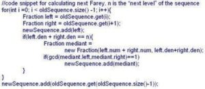
Below is some Java-ish code corresponding to the above – it assumes that the oldSequence and newSequence are an ArrayList and that you have a class Fraction that has fields num (numerator) and den (denominator).

Here are the first five Farey sequences that you get from the algorithm:

The image at the top of the post was generated by implementing the algorithm in Processing, and using the result to draw the associated Ford circles – you could do something similar in regular Java (or other language). If you draw the Ford Circles associated with the sequence, the circle for a fraction “frac” will be centered at (x,y) and have a radius r where

x = (scale)*frac.num/frac.den

y = r

r = (scale)/(2*(frac.den)^2)

where “scale” is some scaling factor (probably in the 100’s) that increases the size of the image.

Here I decided to draw two copies of each circle, one on top of the other.

 

That it contains only fractions between 0 and 1 and that it contains all reduced fractions for denominators k < n, connects Farey sequences to Euler’s totient function. Euler’s totient function is an arithmetic function that for a given k, counts the integers less than k that are relatively prime to it. This is exactly the number of times that a fraction of the form h/k will appear in the Farey sequence for k>1.

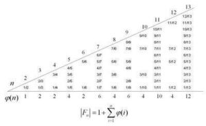
The Farey algorithm, how to draw Ford circles, and the connection to Euler’s totient function are described nicely in J.H. Conway and R.K. Guy’s The Book of Numbers – a great companion to a book like TofN.

 

For more such insights, log into www.international-maths-challenge.com.

*Credit for article given to dan.mackinnon*

 

Chapter 3 of Hardy & Wright’s An Introduction to the Theory of Numbers involves Farey sequences – which, in addition to showing up in serious number theory books, are an interesting, accessible, and popular topic in recreational mathematics.

Since I am a committed constructivist (in at least a few senses of the word) I thought it would be nice to come up with an activity with Farey sequences that could be carried out without too much advance discussion about what they are. What I came up with is a Fathom activity that starts with some simple but odd looking data that allows you to construct some very interesting plots and displays. The idea is that you will get a feel for what a Farey sequence is by using the data to build the sequence and by looking at the results from different perspectives.

Step 1. Import some data

Here is the data to import into Fathom. It should create 33 cases with two attributes n, and d.

n d

0 1

1 10

1 9

1 8

1 7

1 6

1 5

2 9

1 4

2 7

3 10

1 3

3 8

2 5

3 7

4 9

1 2

5 9

4 7

3 5

5 8

2 3

7 10

5 7

3 4

7 9

4 5

5 6

6 7

7 8

8 9

9 10

1 1

 

Step 2. Add some more attributes

After importing this data, you should create the following attributes

i = caseIndex

q = n/d

dist = q – prev(q)

mediant = (n+prev(n))/(d+prev(d))

d_mediant = mediant – prev(mediant)

disp = concat(n,”/”,d)

The meaning of the “mediant” attributes will become clearer after you read about Farey sequences.

 

Step 3. Explore some plots

Plots you could try creating are:

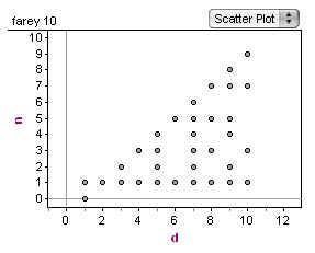
1. A) n on the y axis and d on the x axis.
2. B) dist on y, i on x (a filter of i>1 makes sense here)
3. C) d_mediant on y, i on x (a filter of i>2 makes sense here)
4. D) mediant on y, q on x (adding a function y=x makes sense here)
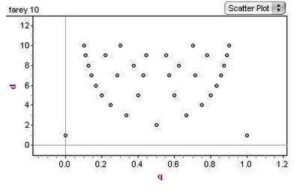
5. E) d on y, q on x
6. F) dist on y, q on x
7. H) q on x with no other attributes

While creating these plots, you should be thinking about describing the sequence that the cases represent. What kinds of numbers are they, what values do they have (do they lie in a certain interval?), how close are they to one another?

Step 4. Create a nice display

One of the more visually interesting thing you can do with the Farey sequence is to display its associated Ford circles. This can be done by adding two new sliders and by editing the display settings for the collection.

 

Add the sliders “scale” and “shift,” and give them these initial values:

scale = 400

shift = 150

Now on the collection inspector, click on the Display tab, and edit the formulas for these attributes

x= q*scale +shift

y = scale/(2*d^2)

image = blueCircleIcon

width = scale/(d^2)

height = scale/(d^2)

caption = “”

If you pull open the display, you will see the initial iterations of a fractal pattern known as the Ford Circles that are generated by the Farey sequence. Here is what it should look like:

For more such insights, log into www.international-maths-challenge.com.

*Credit for article given to dan.mackinnon*

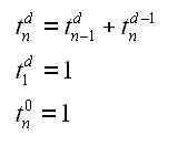
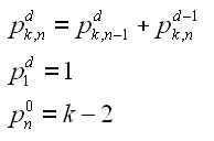
The double recurrence relation that defines the higher triangular numbers is a simple one – it is no surprise that they turn up so often.

The geometric interpretation is stacking: For a given dimension d, you get the n+1 d-triangular number by stacking the nth d-1 triangular number (the gnomon) onto the nth d-triangular number.  The zero dimensional triangular numbers are just the sequence: 1, 1, 1, 1,…, presumably counting stacks of nothing. The one-dimensional triangular numbers are the naturals: 1, 2, 3, 4, …, made by stacking the ones of the one-dimensional case. The two dimensional triangular numbers stack the naturals: 1, 3, 6, 10, …, the three dimensional triangular numbers make pyramids of the triangulars: 1, 4, 10, 20, ….

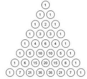
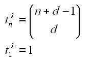
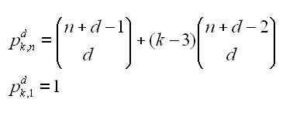
If you write out a difference table for the higher triangular numbers, you end up with Pascal’s triangle. This suggests a nice formula for the triangulars in terms of binomial coefficients:

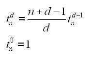
From this, you can obtain another recursive formula that you can use when working with higher triangular numbers (this is the “another” formula for this post):

If you vary the defining recurrence relation so that the initial “zero dimensional” value is a number other than 1, you get the other polygonal numbers (square, pentagonal, hexagonal, square-based pyramidal, etc.). In particular, if you let the zero-dimensional value be k-2, you obtain the k-polygonal numbers (k-2 corresponding to the number of triangles in your k-sided polygon).

It turns out there is a nice formula for these in terms of binomial coefficients as well:

For more such insights, log into www.international-maths-challenge.com.

*Credit for article given to dan.mackinnon*

As I make my way through Hardy & Wright’s An Introduction to the Theory of Numbers,  I am hoping to work it into my recreational math pursuits – coming up with interesting (but not too heavy) activities that correspond roughly to the material in the text.

The first two chapters are on the sequence of primes. Here’s the activity: obtain a list of primes, import them into Fathom, and construct plots that explore pn and pi(n) and other aspects of the sequence that manifest themselves in the first couple of thousand terms.

In my Fathom experiment, I imported the first 2262 prime numbers.

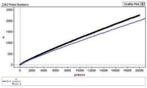
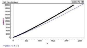
If you import a sequential list of primes into Fathom (under the attribute prime) and add another attribute n=caseindex, you can create two nice plots. Plot A should have prime as the x axis and n  as the y axis. This shows the function pi(n). To this plot you should add the function y = x/ln(x) and visually compare the two curves. Plot B should have the x and y axis reversed. On this graph, plotting the function y = x*ln(x) shows how closely this approximation for pn (the nth prime) comes to the actual values.

 

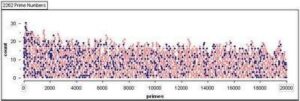
You can add further attributes to look at the distance between primes dist=prime-prev(prime), and also the frequency of twin primes is_twin = (dist=2)or(next(dist)=2).

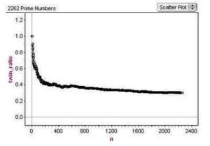
You can also add attributes to keep a running count of twin_primes, and to keep a running average of the twin_primes. The plot above shows how the ratio of tiwn primes diminishes as the number of primes increases. The plot at the top of the post suggests the distribution of primes and twin primes (in blue) in the numbers up to the 2262nd prime.

For more such insights, log into www.international-maths-challenge.com.

Credit for article given to dan.mackinnon*