Month: April 2017

When asked to describe mathematics we often resort to metaphor rather than attempt to provide strict definitions. These pictures from high school math textbooks from the 1930s are an example of this tendancy.

The simple hierarchies of these images resolve the complicated relationship between mathematics and science by appealing to our desire for an organic unity among disciplines, giving mathematics a foundational role within the general concept of science. These images are appealing, but do not stand up to scrutiny.

The simple relationship between mathematics and science becomes complicated when mathematics is described, as it sometimes is, as a science itself. It’s definition as “the science of space and quantity” is further complicated by the caveat that it is an exact deductive science, unlike the usual inductive kind. Following this line of thinking further, mathematics is then described as a kind of meta-science, or a limit point to which science might aspire – science emptied of all of its empirical content, a science of pure thought. While some view mathematics as a foundation for science, others as a supra-science, the emerging field of experimental mathematics brings mathematics back into the empirical fold, reducing it (or elevating it) to a science like any other. So, mathematics can be seen as root, branch, or even the form of the tree itself.

Thinking about these things for even a short while evokes some sympathy with Bertrand Russell’s remark that “mathematics may be defined as the subject in which we never know what we are talking about, nor whether what we are saying is true.”

For more such insights, log into www.international-maths-challenge.com.

*Credit for article given to dan.mackinnon*

Start with a square piece of paper (like a Post it note), fold and unfold it in half along a mid-line or along a diagonal. Take another identical square, and fold and unfold it the same way. Decide on some way to place the second square on the first, so that the second is somewhat rotated. Use only the edges of the square and the creases that you made to determine the placement. Make your placement precise so that your “rule” can be described exactly in terms of the edges and creases. Repeat this process, placing a third square on top of your second square using exactly the same rule. Repeat until your placing of papers leads you back to the first piece.

The resulting construction might look something like the one shown on the left below. If you take your papers, set them in place with some careful light gluing, and place them on a window, the sunlight passing through the overlapping papers creates a stained-glass effect that shows a variety of shapes.

This sort of construction is a simplified version of what William Gibbs describes in his book “Window Patterns.” In Gibbs’ treatment, the pattern is partially planned in advance, and then the dimensions of the rectangular pieces of paper that make up the pattern are determined using a little trigonometry. This process can be simplified by starting with a more limited range of options for paper dimension and placement. It turns out that a surprising number of window patterns can be created by only using squares, their mid-lines, and their diagonals, and that these patterns invariably have “special triangles” and related regular polygons and star-polygons embedded within them.

Here are a two more “placement rules” and the patterns that they give rise to.

The diagrams were created using Geometer’s Sketchpad – if you construct the rule using translations applied to a constructed square, you can use the iteration feature to create the final pattern. GSP provides a good environment for planning out the patterns prior to constructing them with paper, and building the plans in GSP is enjoyable and instructive as well.

For more such insights, log into www.international-maths-challenge.com.

*Credit for article given to dan.mackinnon*

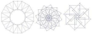
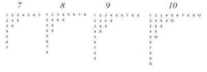
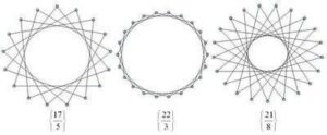
Starting with p (p a positive integer) equally distributed dots (vertices) around a circle. Connecting each dot to the next as you move around the circle will give you a regular p-gon – a p-sided polygon with p vertices. If, however, instead of connecting each dot to the one next to it you skip over a fixed number of dots, then you might end up with a star-like pattern, like the ones shown above. In this process, imagine that you start with a particular vertex and move in a counter-clockwise direction. If there are any dots left-over when you get back to the dot you started from, just throw away the unconnected dots.

The Schläfli notation for polygons is very useful for describing regular connected star polygons, and provides an example of how sometimes calculations with notation match exactly with calculations done with diagrams. In this notation, regular polygons like triangle, square, pentagon, etc. are written as {3}, {4}, and {5} respectively. A regular p-gon is written as {p}. If when drawing your p-gon you connect to the second next vertex instead of the first, then you would write this as {p/2}. If you connect to the q’th next vertex, then you would write this polygon as {p/q}. Note that if you are just connecting to the next vertex to make a regular p-gon, this notation gives you {p/1} = {p}, as you would expect.

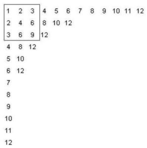
If you start playing with this process you will notice that {p/q} gives you the same polygon as {p/(p–q)} (as long as you ignore the orientation of the polygon). You may also notice that if q is larger than p, you end up repeating the same patterns, in particular {p/q} = {p/(q mod p)}. Also you will notice that if p and q have common factors, you end up having skipped vertices. In our process we are throwing these away to ensure that our polygons are connected, but you can extend the process and keep them (see note below).

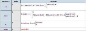
The process described is straightforward to implement in a program. The images shown here were generated in Tinkerplots. To implement it in Tinkerplots, you need two sliders – p and q, and the following attributes:

n = caseIndex()
theta = 2*n*pi(1-q/p)
x = cos(theta)
y = sin(theta)

If you create a plot with y vertical and x horizontal, choose “show connecting lines” and add a filter n<=p+1, you can add a large number of cases to the collection (~200, say) and be able to slide p and q to create a wide variety of connected star polygons. The only restriction is that p must be less than the number of cases you have created. There is nothing special about using Tinkerplots here – any programming environment with reasonable graphics should do a reasonable job (Logo would be fine. :)).

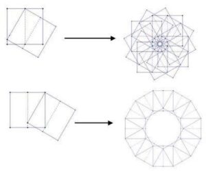
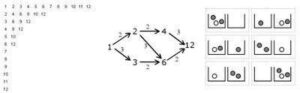
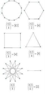
The polygons below are the regular connected polygons based on 12 vertices. Because 12 is divisible by 2, 3, 4, and 6 we end up with regular polygons triangle {3}, square {4}, hexagon {6} and only one star polygon {12/5}. The “degenerate” polygon {2} is known as a “digon.” Here, drawing the diagram first and then seeing what polygon comes out will give you the same result as dividing p/q first and then drawing the corresponding polygon. In this sense, the notation and diagrams nicely reflect each other.

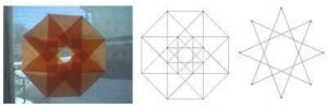
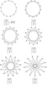
Contrast this with the family of star polygons that are generated when a prime number of vertices are used. The images below are the family of regular connected polygons generated on 13 vertices.

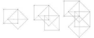
Note – by throwing away the unconnected dots in our process we are ignoring star polygons that are made of overlapping disjoint star or regular polygons, for example two overlapping triangles that make a star of David. These also work well with the Schläfli notation. To create these overlapping polygons, if you have any skipped vertices, you just begin your process again beginning with one of the vertices you skipped over. In the case of {6/2}, instead of getting one triangle {3} you will get two overlapping triangles, or 2{3}. To write a program that would draw these you would want to use something more sophisticated than Tinkerplots.

For more such insights, log into www.international-maths-challenge.com.

*Credit for article given to dan.mackinnon*

A surprisingly interesting structure is the extended multiplication table, shown above for the numbers seven to ten. The algorithm for drawing these is straight forward – for an n-extended table, start out as if you were writing a “regular” multiplication table, but extend each row so that it gets as close to, without exceeding, n. Another way to think about it is to write out rows of “skip counting up to n” by i for integers i from 1 to n.

This is called an extended multiplication table since it contains a “traditional” multiplication table inside it. The 12-extended table below contains a traditional 3×3 multiplication table.

It turns out that 1 appears in an extended table once, and prime numbers appear exactly twice (once in the first column, and once in the first row). In general, for a natural number n, how many times does n appear in the n-extended table?

Before looking at that question, you might want to think about finding easier ways to draw the tables. Drawing out these tables by hand can be tedious – a simple program or spreadsheet might be easier. You can use Fathom, for example, to create the table data and draw it in the collections display. Create a slider m and the attributes listed in the table below (click on the image to see a larger version).

Modify the collection display attributes to draw the tables in the collection box. By adding lots of cases and using the slider m to filter out the ones you don’t need, you can vary the size of the table easily.

“how many times does n appear in the n-extended table?”

# of occurrances of n in the n-extended table = # of nodes in the factor lattice Fn

You can also recast both of these questions (how many occurances of n in the n-extended table, and how many nodesin the Fn factor lattice) as a combinatorial “balls in urns” problem.

Consider a set of colored balls where there are m different colours, where there are ki balls of color i, where i ranges from 1 to m. This would give a total number of balls equal to k1+k2+…+km. Suppose you were to distribute these balls in two urns. How many different distributions would there be? Using some counting techniques, you will find that the answer is (k1+1)*(k2+1)*…*(km+1).

How is this connected to the other problems? Consider the prime factorization of the number. For each prime, choose a colour, and for each occurance of the prime in the factorization, add a new ball of that color. For example for 12 = 3*3*2, choose two colours – say blue=3 and red=2. Since 3 occurs twice and 2 occurs once, there should be two blue balls and one red ball. Now consider distributing these balls in two urns. It turns out that you get (2+1)*(1+1) = 6 possibilities. This is the same number of times 12 occurs in the 12-extended table, and the same number of nodes in the 12-factor lattice. The image below shows the 12-extended table, the 12-factor lattice, and the “ball and urn problem” for the numer 12.

For a number n with the prime factorization:

The answer to all three questions is given by:

For more such insights, log into www.international-maths-challenge.com.

*Credit for article given to dan.mackinnon*