Month: February 2017

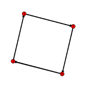
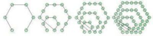
Polygonal numbers are a mainstay of recreational and school mathematics, providing a nice bridge between numbers and shapes. The diagrams above show some of the hexagonal numbers.

Some examples of two-dimensional polygonal numbers are:

the triangular numbers: 1, 3, 6, 10, 15, …
the square numbers: 1, 4, 9, 16, 25, …
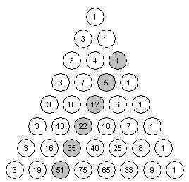
the pentagonal numbers: 1, 5, 12, 22, 35,…
the hexagonal numbers: 1, 6, 15, 28, 45, …

Comparing the listing for the hexagonal numbers with the diagrams above, you can see how the sequences are built diagrammatically. In general, beginning with a single dot, k-sided polygons are built by adding layers (called gnomons) consisting of k-2 segments, with each segment of the gnomon having one more dot than the segments of the previous layer. In this way, the nth gnomon consists of segments each n dots long, but with k-3 dots shared by adjoining segments (the corners).

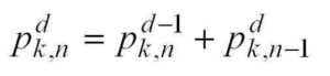
The description above can lead you to a recursive formula for k-polygonals, writing p_k,n for the nth k-polygonal number:

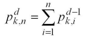
Unwinding the recursion gives you a summation formula for k-polygonals:

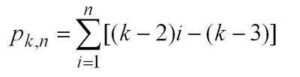
Knowing a little about sums gives you the direct formula for k-polygonals:

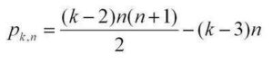
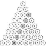
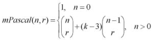
Coming a little out of left-field is this combinatorial formula for k-polygonals:

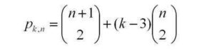
This last formula expresses two ideas: that the triangular numbers correspond to the r=0 column of Pascal’s triangle, and that every polygonal number can be “triangulated”:

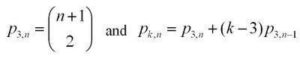
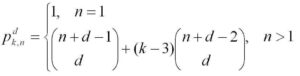
The combinatorial formula for p_kn can be generalized to higher-dimensional polygonal numbers (pyrimidal numbers, etc.).

The recreation here lies in showing that the various formulas for p_k,n are really the same, and then exploring the relationships between the different k-polygonals. A great resource is J.H. Conway and R.K. Guy’s The Book of Numbers.a

For more such insights, log into www.international-maths-challenge.com.

*Credit for article given to dan.mackinnon*

Sonobe and phizz modular origami units are assembled into polyhedral models in similar ways, but the models that they produce are “dual” to each other (vertices in one correspond to faces in the other). Assembling models out of sonobe and phizz units with this duality in mind provides a nice way of exploring duality and the relationships between edges, faces, and vertices.

The sonobe and phizz modules are both examples of edge modules that come together in groups of 3. In both cases, when the units come together in their groups of 3 they meet in a small triangular pyramid. These pyramids in turn come together in clusters of 3 to 6. The essential difference between the phizz and sonobe modules is in how these clusters form. In the phizz, there is a gap between the groups, so the resulting cluster seems to form the edges of a polygon. In the sonobe, the gap between the groups is small, so the cluster seems to form around a point. Consequently, in the phizz, the center of the cluster takes on the role of a polygonal face, while in the sonobe it is takes on the role of a vertex. Meanwhile, the pyramids formed by the groups of three units become raised vertices in the phizz unit, while in the sonobe they become cumulated faces of the resulting polyhedron.

We naturally interpret what phizz modules generate as polyhedral skeletons, while we see the shapes generated by sonobe as cumulated (or augmented) polyhedra. The fact that this different interpretation is based on the size of the gap that forms in the center of the module clusters suggests that seeing an origami model as a particular polyhedron or its dual is, to some extent, a matter of perception and interpretation.

In phizz models, the fact that the modules come together in groups of 3 dictates that the finished models have vertices of degree (or valence) 3, while in the sonobe case, the 3 units come together to make triangular faces. Dual models have the same number of edges, which corresponds to the number of modules required to build the model.

Some of the models that you can build are summarized below. The picture at the top of the post shows the 30-unit phizz dodecahedron and its dual, the 30-unit sonobe icosahedron.

For more such insights, log into www.international-maths-challenge.com.

*Credit for article given to dan.mackinnon*

Looking at the last few digits that appear in the numbers that form the sequence b^0, b^1, b^2, b^3, … for b a positive integer, you’ll notice that the digits will always begin to repeat after a certain point. For example, looking at the last digit of the sequences for b = 2, 3, and 4 we have the sequences

b = 2: 1, 2, 4, 8, 6, 2, 4, 8, 6, …
b = 3: 1, 3, 9, 7, 1, 3, 9, 7, …
b = 4: 1, 4, 6, 4, 6, 4, 6, …

If we look at the sequence of last two digits of these sequence where b =2 we have

b = 2: 1, 2, 4, 8, 16, 32, 64, 28, 56, 12, 24, 48, 96, 92, 84, 68, 36, 72, 44, 88, 76, 52, 4, …

This sequence then repeats the loop that began at 4.

We can describe these sequences as T_b,d(n) = (b^n)mod 10^d. Recursively, T_b,d(n) = (T_b,d(n-1)*b)mod 10^d

These sequences are always eventually periodic. Although these sequences are simple to understand and calculate, there are several interesting ways of describing them.

For example, you can think of the elements of T_b,d as a commutative monoid, with multiplication defined as a*b = (a*b)mod 10^d. They form a monoid since 1 is always a member, and you can show that T_b,d is closed under the * operation. It turns out that for some values of b, and d, T_b,d is a group.

You can also think of this set as a finite state machine or graph, where each element is a node and the transition from one node to the next is defined by the operation *b mod 10^d. This provides a nice way of displaying the sequences. The pictures in this post were created by writing a short program to calculate the sequences, and then formatting the output to draw a di-graph in SAGE. The graph at the top of the post is for b=8, d=1, while the graph below is for b=2, d=2. The graph at the bottom of the page is for b=7, d=1.

For more such insights, log into www.international-maths-challenge.com.

*Credit for article given to dan.mackinnon*

The third diagonal column in Pascal’s Triangle (r = 2 in the usual way of labeling and numbering) consists of the triangular numbers (1, 3, 6, 10, …) – numbers that can be arranged in 2-dimensional triangular patterns. The fourth column of Pascal’s triangle gives us triangular-based pyramidal numbers (1, 4, 10, 20, …), built by stacking the triangular numbers. The columns further out give “higher dimensional” triangular numbers that arise from stacking the triangular numbers from the previous dimension.

It is not by coincidence that the triangular and higher-dimensional triangular numbers appear in Pascal’s Triangle. If you think about layering of polygonal numbers in terms of equations, you get

In the above equation p^d_(k,n) is the nth k-polygonal number of dimension d. Triangular numbers are the 3-polygonal numbers of dimension 2, square numbers are the 4-polygonal numbers of dimension 2, “square based pyramidal numbers” would be denoted as p^3_(4,n).
from the sum above, you can obtain this equation:

Which looks very much like the Pascal Identity C(n,r) = C(n-1,r-1) + C(n-1,r), except for some translation of the variables. To be precise, if we consider the case where k=3 and use r = d and n‘ = n+d-1 we can translate the triangular numbers into the appropriate positions in Pascal’s Triangle.

Along with the definitions for the end columns, the Pascal Identity allows us to generate the whole triangle. This suggests the following strategy for calculating the higher k-Polygonal numbers: create a modified Pascal’s Triangle whose first column is equal to k-2 (instead of 1), and whose last column is equal to 1 (as usual). This modified Pascal’s Triangle is generated using these initial values and the usual Pascal Identity.

Here is an example with k=5, which sets the first column values equal to 3 (except for the top value, which we keep as 1) and yields the pentagonal numbers (column 3) and the higher pentagonal numbers.

The formula for these modified Pascal Triangles is given by this equation:

If we apply the change of variables mentioned above, we can obtain this general formula for the higher polygonal numbers in terms of combinations:

This formula illustrates how polygonal numbers are built out of triangular numbers. It says that the nth d-dimensional k-polygonal number is equal to the nth d-dimensional triangular number, plus (k-3) copies of the n-1 d-dimensional triangular number. This is a little easier to understand when you forget about the higher-dimensions and look at the regular 2-dimensional polygonal number.

For more such insights, log into www.international-maths-challenge.com.

*Credit for article given to dan.mackinnon*