With connections to the study of gambling, Brownian motion, fractals, and more, random walks are a favourite topic in recreational mathematics.

The diagram above (from Energy transformations during horizontal walking by F. G. Benedict and H. Murschhauser, published in 1915) suggests one method for generating walking data. Creating random walk simulations in Fathom or TinkerPlots is a little more straightforward.
First simulation – using sliders to determine a ‘base angle’
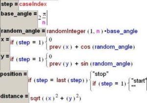
This first example lets you set up random walks where the direction chosen is based on an angle k*2pi/n for a fixed n (whose value is determined by a slider) and a random k (a random integer between 1 and n).
First, create a slider n, then create the attributes below and finally add the data (any number is fine – start with ~500 cases). The formulas below were entered in TinkerPlots, but would work equally well in Fathom.

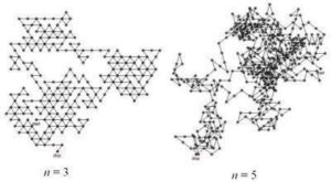
Plots of (x,y) will show the walk, and plots of (step, distance) will show how the distance from the origin changes over the course of the walk. Different values for n provide walks with their own particular geometries.

The walks start at (0,0) and wander about the plane from there. Re-randomizing (CNTRL-Y) generates new walks.
The simulation gives lots of nice pictures of random walks. You could generate statistics from these by adding measures and measure collections.
One limitation of this simulation is that it is difficult to determine exactly when the walker has returned to the start (0,0). This turns out to be an interesting question for random walks on the plane (see the wikipedia entry for more on this). Because of the inexactness in the positions calculated using sine and cosine, the walker seems to never return to the origin. There are several ways of dealing with this, but one is to design a simpler simulation that uses exact values – one that sticks to lattice points (x, y), where x and y are both integers.
Second simulation – sticking to Integer lattice points
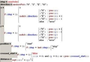
This second simulation can be thought of an ‘urban walker’ where all paths must follow a strictly laid out grid, like some downtown streets. The exactness of the positions means that we can detect with confidence when the walker has crossed back to their starting point. For this simulation, no slider is required – just enter the attributes and add cases.

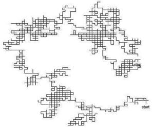
Using the crossed_start attribute as a filter or to gather measures, you will find that walks often quickly pass over the starting point. You will also find that as you increase the number of cases, the straight ‘etch-a-sketch’ lines of the urban walk take on very interesting fractal-like contours.

For more such insights, log into www.international-maths-challenge.com.
*Credit for article given to dan.mackinnon*

