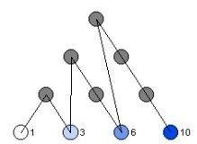
The diagram above (known as the tetractys) shows the first four triangular numbers (1, 3, 6, 10, …). Although there is a simple formula for calculating these numbers directly, t(n) = 1/2(n(n+1)), constructing them by these layered-triangle diagrams helps to show their geometric and recursive properties.

More generally, polygonal numbers arise from counting arrangements of dots in regular polygonal patterns. Larger polygons are built from smaller ones of the same type by adding additional layers of dots, called gnomons. Beginning with a single dot, k-sided polygons are built by adding gnomons consisting of k-2 segments, with each segment of the gnomon having one more dot than the segments of the previous layer. In this way, the nth gnomon consists of segments each n dots long, but with k-3 dots shared by adjoining segments (the corners).
This post describes how you can draw figures that illustrate the polygonal numbers and explore the polygonal numbers in general (triangular, square, pentagonal, hexagonal, etc.) using either TinkerPlots or Fathom. Both TinkerPlots and Fathom work well, but TinkerPlots creates nicer pictures, and allows for captions directly on the graph.
Without describing the details of how you create Fathom or TinkerPlot documents, here are the attributes that you will want to define in order to draw diagrams like the ones shown.
Required attributes
Create a slider k. This will allow you to set what kind of polygonal number you want to draw (k=3 gives triangular numbers, k=4 gives square numbers, etc.)
Define the following attributes:
n The number itself. This is a natural number beginning at 1 and continuing through the number of cases.
gnomon This states which “layer” or gnomon the number belongs in. It is calculated based on a number of other attributes.
g_index This is the position of the number within the gnonom – it ranges from 1 up until the next k-polygonal number is hit.
s_index Each gonom is broken up into sections or sides – what is the position within the side? Each side is of length equal to the gonom number. The first gonom has sides of length 1, the second has length 2, etc.
corner This keeps track of whether or not the number is a “corner” or not. This is based primarily on the s_index attribute.
c_index This keeps track of how many corners we have so far. There are only k-1 corners in a gnomon (the first number n=1 is the remaining corner). So, when we hit the last corner, we know we are at a polygonal number.
k_poly Records whether or not the number n is k-polygonal. It does this by checking to see if it is the last corner of a gnonom.
The attributes listed above are required for finding the position of each number within the figure; th following attributes are used in actually drawing the figures.
angle The base corner angle for the polygon is determined by k. This is the external angle for each corner.
current_angle We have to add to the base angle at each corner as we turn at each corner. This attribute is used to keep track of the total current angle.
dx This is the x-component of the unit direction vector that we are travelling in. Each new dot moves one dx over in the x-direction. It is given by the cosine of the current angle.
dy This is the y-component of the unit direction vector that we are travelling in. Each new dot moves one dy over in the y-direction. It is given by the sine of the current angle.
prev_g_1_x This is the x-coordinate of the first dot in the previous gonom layer. We need to know this because it will be the starting point for the next layer – each layer starts back at the “beginning” of the figure.
prev_g_1_y This is the y- coordinate of the first dot in the previous gonom layer.
x This is the x-coordinate of the current dot, calculated either from the previous dot or from the first dot in the previous layer.
y This is the y-coordinate of the current dot, calculated either from the previous dot or from the first dot in the previous layer.
caption Used to display the number on the plot (TinkerPlots only)
Below are the formulas for each attribute, written in “ascii” math. They are presented without a full explanation, in the hopes that if you try to implement this you will think about and explore each using the formulas and the descriptions above as a guide. Alternate methods for drawing the diagrams are possible, and you might find other formulas that achieve the same goals. Note that there are nested if() statements in several formulas.
n = caseIndex
gnomon = if(n=1){1, if(prev(k_poly)){prev(gnomon)+1, prev(gnomon)
g_index = if(n=1){ 1, if(prev(k_poly){1, prev(g_index) +1
s_index = if(n=1){ 1, if(prev(k_poly){1, if(prev(s_index) = gnomon){2,prev(s_index)
corner = (s_index=1) or (s_index=gnomon)
c_index= if(g_index=1){1, if(corner){prev(c_index)+1, prev(c_index)
k_poly = if(n=1){true, (c_index=k-1)
prev_g_1_x = if (n=1){0, if(g_index=2){prev(x), prev(prev_g_1_x)
prev_g_1_y = if(n=1){0, if(g_index=2){prev(y), prev(prev_g_1_y)
angle = pi-((k-2)*(pi/k))
current_angle = if(g_index =1) {pi-angle, if(pref(corner)){prev(current_angle)-angle, prev(current_angle)
dx = cos(current_angle)
dy = sin(current_angle)
x= if(n=1){0, if(g_index=1){prev_g_1_x +dx, prev(x) +dx
y =if(n=1){0, if(g_index=1){prev_g_1_y +dy, prev(y) +dy
caption = if(k_poly){n,””
To actually draw the diagrams, create a new plot with the x and y attributes as the horizontal and vertical axis, respectively. Add cases to the collection to populate the diagram. Optionally you can show connecting lines, and (in TinkerPlots) add a legend using the caption attribute.

For more such insights, log into www.international-maths-challenge.com.
*Credit for article given to dan.mackinnon*

